In my AU library, I offer some utilities related to curves. Although Processing offers functions for finding points on curves, I needed to write my own implementation that was fast and efficient. Here’s an easy, elegant way to compute points on Catmull-Rom and Bezier curves, along with a discussion of an idea for making it faster.

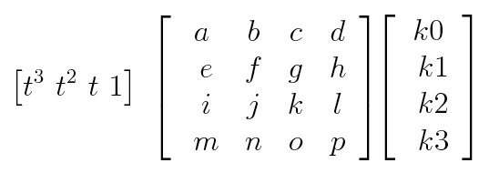
The most convenient way to generate points on these curves is to use a matrix form, as nicely summarized by Tom Duff’s memo. Suppose we have a curve with knot values k0, k1, k2, and k3. Form them into row vector, which I’ll call k. We’ll be using this in column form, so I’ll use this vector in its transposed form, written k^T. Now we want to find a point at the parameter value t along the curve. Form a row vector as [t³ t² t 1], which I’ll call t.

To find the value of the curve at t, we need only one more thing: a 4-by-4 matrix, which I’ll call M. This matrix sits between the two vectors as in the tableau above. Multiplied together, these three elements give us the scalar t M k^T, which is the value of the curve of matrix type M, with knot data k, at time t. Each particular kind of curve has its own characteristic matrix M that combines t with k in the just the right way.

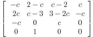
Cardinal Spline Matrix

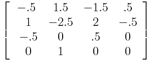
Catmull-Rom Matrix

The interesting thing is that we can use this form for both Bezier curves and all the cardinal splines. The cardinal splines take a single parameter, which Duff calls c. When c=0 we get straight lines from knot to knot, and when c=.5 we get Catmull-Rom curves. Values of c between those values blend between the polygon and Catmull-Rom forms. Values of c outside that range produce very squiggly curves.

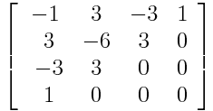
A nice derivation of the matrix form of the Bezier curve is described by Ken Joy here (note that Joy writes his t vector in the opposite order that I’ve written it, so I’ve flipped his matrix to make it match our notation).

Bezier Matrix

To evaluate a 1D curve at t, we just put our knot values into k, build t, and evaluate t M k^T. Because these curves are independent along each axis, we can blend as many values as we like for each value of t just by changing k. For example, to evaluate a 2D curve, with knot values for X and Y, we only need fill up k with the X values, and find t M k^T. To find the Y value, just put the Y values into k and find t M k^T again. We can attach other data to each knot, such as stroke thickness or rainfall that day, and interpolate it as well.

This suggests saving some time by computing t M just once for a given value of t, and then applying it to each different set of k.

But wait, why not pre-compute t M for all time? Then for any given value of t, we find the two closest pre-computed vectors, linearly interpolate them, and then apply them to k. For example, save a static table tMtable[1000][4], loaded with the 4-element vector t M for 1000 choices of t. When a value of t arrives, find the two indices that bracket it, which I’ll call i0 and i1. We’ll say that b is a float from 0 to 1 across that interval, telling us where t lands. Then we can find the value of t M, which I’ll save in a 4-element vector tM:

for (int i=0; i<4; i++) tM[i] = lerp(tMtable[i0,i], tMtable[i1,i], b);

Great, now we have tM holding t M, and we can find the spline value by just dotting it with the vector k holding our knot data:

float val = 0;
for (int i=0; i<4; i++) val += tM[i] * k[i];

I like this idea, but is it worth it? Writing out the full evaluation of t M k^T, we’d need 20 multiplies and 5 adds. In this lookup table form, we’d need a total of 8 multiplies and 12 adds (and that’s leaving out the overhead of the loops, and finding the values of i0, i1, and b). Unfortunately, this doesn’t seem at all worth it. Finding t M just isn’t that expensive.

I think it’s always worth looking at these kinds of time/space tradeoffs, because they often return impressive benefits. But it’s important to look at them closely, so we don’t waste time implementing “optimizations” that aren’t optimizing anything!