Solving Geometry Problems
Andrew Glassnerhttp://The Imaginary Institute
8 May 2013
andrew@imaginary-institute.com
https://www.imaginary-institute.com
http://www.glassner.com
@AndrewGlassner
Imaginary Institute Tech Note #1
When writing graphics programs, you frequently need to dream up little bits of geometry to make things look just right. While writing a program last night, I needed to figure out how to draw a shape that I wanted. It was all about geometry: given the kind of shape I wanted to make, what do I have to draw to create it? I remember solving just this geometry problem years ago (and even printing it in a book!), but I thought it would be more fun (and save me a trip downstairs to get the book) to work it out again.
Note that this discussion will bring in a little bit of trigonometry, or just "trig". Imaginary Institute Technical Note #2 covers what you need to know if you've forgotten (or never learned) what sine and cosine and all those things are about. If you're hazy on that stuff, for now just gloss over the details when it gets used. They're great tools that you'll definitely find handy, so I suggest that you do eventually brush up on them.
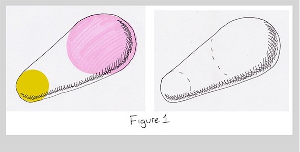
I was working on a 3D project. In this project I had pairs of spheres of different radii, and I wanted to put a cone between them that would *smoothly* blend them together, like in this sketch:
As I looked at this problem, I realized that after doing thousands of this kind of thing I've developed process for solving them. Of course, lots of people have written about how to solve all kinds of problems, from scriptwriting to dishwasher repair, so I don't claim to have anything unique to offer here. But I hope that by sharing how I go about solving something like this, it might help you develop your own approach. I thought this was a good problem to use, because it's a useful result that came up in a real project, and the answer isn't immediately obvious (at least, it wasn't to me).
Now I love 3D, but it can be a tough place to do geometry. I realized I could express this much more simply if I just thought about it as a cross-section. Then I have a 2D problem, not 3D. The goal is now to find the lines that smoothly join up two circles, like this:
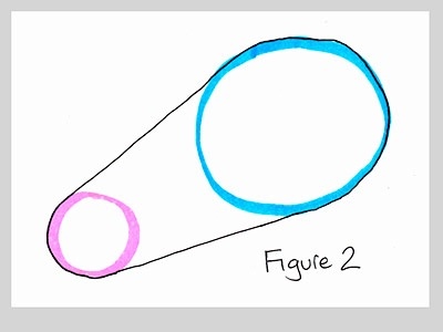
Note that these lines are not just straight lines through the circle centers; that is, they're not diameters. Here's what it looks like if you use diameters:
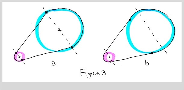
b) If we compute the points properly, the circles join up smoothly.
Not smooth. Not good. So the question now is how to find the points on the two circles that will do the job of smoothly blending them together.
If you're in the heat of writing a program and you just need the answer, you can skip down and find it at the end. We're going to go slow because I want to demonstrate to you the *process* of finding an answer.
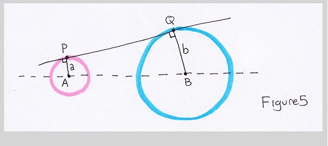
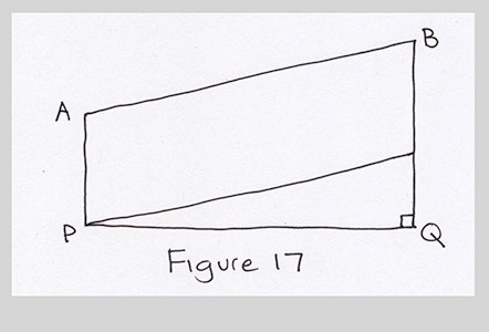
First, I labeled everything. The point at the center of one circle I called A, and its radius a. The other circle is centered at B, and it has radius b. For convenience, I'll just call the first circle A and the second one B (note the boldface type when I'm referring to the circle rather than the point at its center - this is a standard trick in mathematical notation that lets you re-use a symbol in multiple ways, so we can imply a connection between them. Here, circle A has center A and radius a). The point I'm looking for on A is called P, and the point on B is called Q.
Here's a picture of where they go:
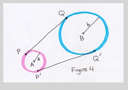
So now the job is to find points P and Q.
Here's the key thing to know: the solutions you find online for this sort of problem (or almost any kind of problem) are the cleaned-up, final results after people have tried a bunch of things. As noted by the mathematician Gauss, a mathematical result is often something that was created through a messy construction process, and then had all the scaffolding stripped away, leaving just the beautiful final result. What you don't see are all the dead ends, blind alleys, and attempts that just didn't work out. People don't show you the pages of paper with equations and drawings that ended up in the garbage, or the code that produced completely broken pictures. They go through all of that, of course, because everyone does. But once they find a nice answer, they work on it to make it as clean and clear as possible, and that's what they share with you.
This is a great way to share information. You give people just the information that they need, and you give it to them as directly as you can. But the beautiful, clean result doesn't give you any clue about how many dead ends the author followed first, or how many times he or she followed a hunch that didn't pay off, or just went off on a completely wrong direction for a while. So the final result can seem intimidating: here's the problem, here's the answer, ta-da!
Geometry problems are often that way, too: you try this, you try that, maybe you have a hunch about something, and most of the time it just doesn't go anywhere. You just end up "discovering" things you already know, like that point A is equal to point A, or that 1 is not 0. Exciting stuff like that. And then finally you stumble on an approach that does work, and that's your solution! If you're like me, you then throw away all those pages you littered with false starts, and save just the page with the right answer (or at least an answer).
So here's what I did last night, warts and all. I definitely didn't get to the right answer right away, even though I've actually solved (and even published!) this very bit of geometry many years ago. I'd forgotten (or it sure felt like I'd forgotten), and had to start from scratch
First things first: write down everything we know. In this case, all we know are the centers A and B, and the radii $a$ and $b$. That's it. Whatever our answer is, it can only depend on these four pieces of input (and values we derive from them).
I started by deciding that circle A would always be smaller than circle B. I'd leave it up to my program to swap the inputs if $a$ was bigger than $b$. I also drew the circles so that their centers were on the same horizontal line - that just made it easier to draw pictures. I sketched the line I wanted to find, and marked the points P and Q.
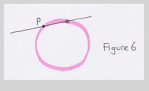
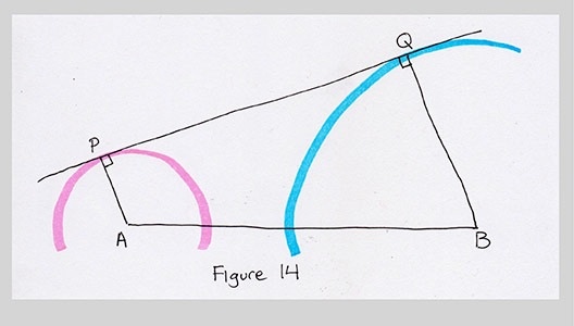
I did one more thing, and that was to put little right-angle boxes at points P and Q, between the line PQ and the radius of each circle. That's because I knew that in order for the line PQ to smoothly join the circles, it had to just kiss, or just graze, each circle at one point. The only line that does that is a line that's perpendicular to the radius. If the line isn't perpendicular to the radius, then it'll intersect the circle at two points, like this:
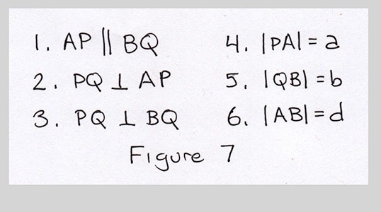
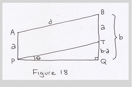
Looking at Figure 5, I noted that the line AP was parallel to BQ (entry 1 in Figure 7). Next, I wrote down that line PQ was perpendicular to line AP. By the same reasoning, line PQ is perpendicular to BQ. Then I noted that the length of line PA (written |PA|) was the radius $a$, and then length of PB was the radius $b$. Finally, I gave the name $d$ to the distance from A to B (that is, the length of line AB).
Great, I have these six little relationships. And what do they get me?
Nothing. Zip. I'm sure the answer's in those six little relationships somewhere, but I didn't see anything jumping out at me (by the way, there are computer programs called constraint solvers that could take these six relationships and give you back the values of P and Q in terms of the circle centers and radii, but let's continue solving this one ourselves).
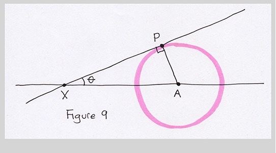
So I tried another approach. What if I extended the line PQ all the way until it crossed the line AB?
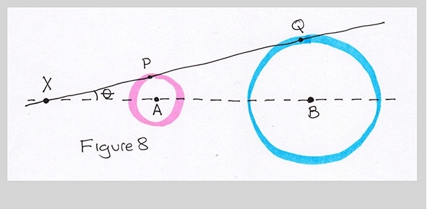
I'll label the intersection point X, and the little angle there as $\theta$ (its traditional to use Greek letters for angles, and theta, written $\theta$, is a common choice). And what has this brilliant little bit of picture drawing done for me?
Nothing. I don't see how this helps anything.
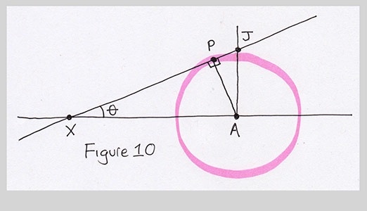
Oh, wait. let's zoom in around points X, P, and A. That's a right triangle. When you have one right triangle, it often helps to look for more, because you can propagate information from one triangle to another to another until you find something useful.
What's that get us? I'm not sure. But since point A is important, lets look in that neighborhood. I'll draw the right triangle on the other side of line AP. So I drew a line from A, perpendicular to AX (so it's also perpendicular to AB), and extended up to line PX. The intersection I called J, and I marked the little angle as a right angle by drawing a little box on that side of P as well.
Um, ok. That's not much help. Let's try one more time. As I said, drawing lots of these right triangles can sometimes lead to something. I'll draw a line from P parallel to XA. It will of course be at right angles to AJ, creating another little right triangle PJK. Since all the sides of this little triangle are parallel to all the sides of the big triangle XJA, I know the little angle in there is also $\theta$.
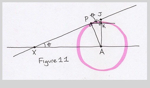
And that helps us... not at all. We have a mess of triangles, but we still don't know anything new. Maybe it's time to ditch this triangle stuff and look for something new to follow. But wait, before we give up, notice that we have yet another right triangle here, PKA. And so the angle at point A is also $\theta$.
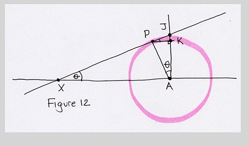
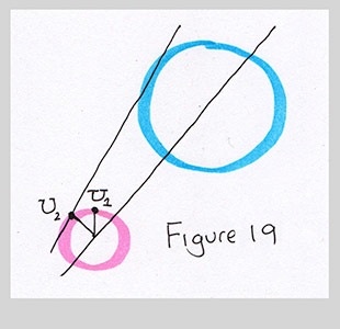
This is good! Because it says angle $\theta$ really is what we want. If we can find $\theta$, then we can find the point I've labeled U in the next figure (on the line through A, perpendicular to AB, at a distance of a from point A), and we can rotate it counter-clockwise around A by to get P. We just saw how to make U from nothing but our inputs. So if we do manage to find $\theta$, then we can use this little recipe to make P (and Q, on circle B) and we're done.
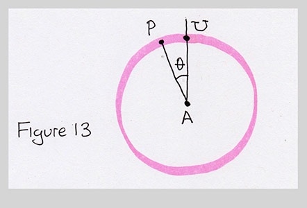
You might be wondering why the same angle can be used for circle B. If you think about it, it has to be the same angle for both circles. Remember that the line can only just graze each circle, so there can be only one point of contact between the line PQ and the circle B, and that's point Q. This also means that the line is perpendicular the radius BQ. So lines AP and BQ are parallel to one another (as we noted earlier), and thus both P and Q are at the same angle with respect to the perpendicular to AB.
If this seems mysterious to you, nothing beats getting out some scratch paper and making a few drawings for yourself. You'll soon convince yourself that these angles have to be the same. That's what did it for me: actually drawing the pictures showed me how the pieces fit together. Do be careful when making these little drawings not to let your eye trick you. Two lines that might seem "obviously" perpendicular, or parallel, or of equal lengths, might only seem that way because they're close enough in your loose drawing that you get fooled. Confirm each relationship logically and don't label anything you're not sure of (by the way, everyone violates this rule now and then, and often regrets it. The hardest errors to catch are the ones that are "obviously" correct!).
That's great. At least now we know what to aim for: the angle $\theta$.
But how can we find $\theta$? I don't know. Let's mess around some more.
Making things simpler sometimes helps, so I redrew the shape made by the four points A, B, P, and Q all by itself. Now what?
Oh, this is interesting. This looks like a quadrilateral. Maybe we can say something about the angles or sides. I think it would be easier to take in the figure if I flip it over.
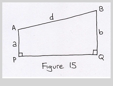
I'd like to make this simpler. Maybe we can break this up into a rectangle and a triangle. Those are easy shapes to work with. What if I draw a line from A, parallel to PQ. It strikes the other vertical line, BQ, at point S. I know that AP has length $a$, so SQ is also a. Since BQ is the radius $b$, I know that the length BS is $b-a$. Great! I've discovered something. I felt pumped.
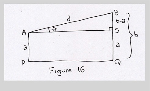
That leaves the little right triangle ABS at the top of the figure. We know that little angle at A from an earlier figure: it's just .
In right triangle ASB, AB is the hypotenuse. Its length is just the distance from A to B, which I called $d$. And side BS has length $b-a$. Basic trig (I did warn you that was coming!) tells us that
$$ d \sin(\theta) = b-a $$We can re-write this to isolate theta:
$$ \sin(\theta) = (b-a)/d $$Now I'll undo the sine function by taking the arc-sin, or asin, of both sides:
$$ \theta = \arcsin((b-a)/d) $$If you're not familiar with "arcsin", this refers to something called the arc-sine or inverse-sine. It's the "inverse function" of the sine. The sine function turns angles into numbers (of course, angles are numbers themselves, too). So if I write sin(30)=.5, I'm giving the number 30 to sine, and (somehow, we don't care how) it gives us back the value .5.
The arc-sine goes the other way, taking in a number and giving us back the angle that, if we gave it to sine, would give us that number. For example, suppose we give arc-sine the number $n$. We'd get back an angle $\alpha$, so that $\alpha = \arcsin(n)$. If we give this value of $\alpha$ to sine, we get back $n$, since $n = \sin(\alpha)$. So $\arcsin()$ lets us "undo" the sine function. Many programming languages and libraries abbreviate this function to asin().
Great! Now we know $\theta$ and we're finished. We could just make the point U as above, rotate it counter-clockwise by $\theta$, and that's P.
Before we proceed, though, let's take another shot at the construction we just made. Sometimes you can find simpler answers if you hunt just a little bit more. So let's take our simplified diagram and follow a different hunch. Instead of drawing a line through A parallel to PQ, let's draw a line from P parallel to AB.
Because ABTP is a parallelogram, and line AB has length d, we know PT has length $d$ also. Because PT is parallel to AB, the segment BT has length $a$, so TQ has length $b-a$. We now have right triangle TPQ, and the angle at P is . Sound familiar?
It's the same triangle as before! We can find $\theta$ by writing $d \sin(\theta) = b-a$, which is the very same relationship we found before, so it leads an identical value for $\theta$. Nothing new, but it was worth taking a shot.
Great, let's wrap it up. In the preceding pictures, finding U was easy: we started at A and moved up by $a$. But that's only because we drew points A and B on a horizontal line, so the perpendicular to line AB went up. When the centers aren't horizontally aligned, the perpendicular to AB is no longer simply up and down:
We could certainly find U anyway, but then we'd still have to rotate it. None of this is particularly hard, but the code can get messy. And if you're not familiar with the technique for rotating a point around another point, it can be kind of mysterious and complicated. Let's try to find a simpler approach.
How about an approach that doesn't involve coordinates at all? We won't even think about x and y values. We'll do it all in terms of vectors, or arrows. We'll start at A, and add a few vectors to it to get P. I'll think in terms of arrows, or vectors (see the video "Arrows", Week 4, Group 2, Video 8). This will give us a really clean answer. The technique is like the one in the video "Using the Geometry" (Week 6, Group 3, Video 5).
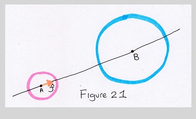
The trick is to break down the location of P with respect to the points A and B. I'll first find the vector J, which is the arrow from A to B. We'll see how to actually compute this in a moment, but for now just think about the pictures. So $J$ is an arrow from A to B, or in symbols, $J$=B-A (I'll write vectors here as capital letters in italics).
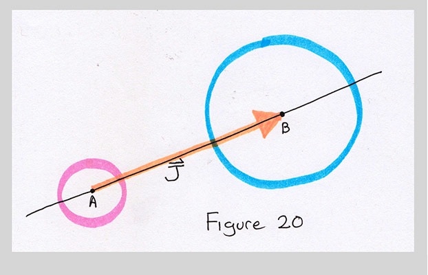
Now I'll normalize that arrow, so it has length 1. This is just a convenience step, because it makes it easy later for us to to scale the vector any length. To show that a vector has unit length, we sometimes place a little hat over it, like this: $\hat{J}$. The hat means a vector of length 1. Since there's no scale yet in my figures, I'll show $\hat{J}$ just by drawing a shorter version of $J$. This actually gives the figures a scale: 1 unit is the length of $\hat{J}$.
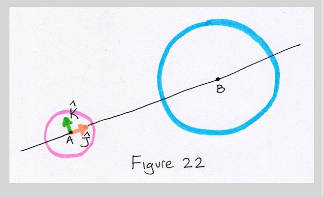
Now I want to find a vector perpendicular to $\hat{J}$. I'll call this new arrow $\hat{K}$. It also has a hat because it also has length 1, and we don't want to forget that useful feature. I'll use our rotate-90 shortcut (see the video "Rotating A Line 90 Degrees", Week 6, Group 3, Video 3) to rotate the vector $\hat{J}$ counter-clockwise by 90 degrees, and thereby get $\hat{K}$.
Now let's look at points A and P. We know that the distance from A to P is $a$. We can draw a little right triangle at A by drawing a line through A in the direction of $\hat{K}$, and another line through P in the direction of $\hat{J}$. The angle at A is just $\theta$.
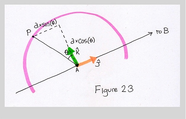
The little triangle tells us how long the two vectors need to be. How much of $\hat{J}$ is required? Just $-a*\sin(\theta)$. What's that minus sign doing there? I want to move the point away from B, but $\hat{J}$ points towards B. So by negating the arrow, I flip it around to point away from B. And how much of $\hat{K}$ do we need? Just $a \cos(\theta)$.
Let's give these names. I'll pick $j_a$ and $k_a$ to remind us that these are scaling $\hat{J}$ and $\hat{K}$ for the circle with center A. I'm using subscripts here just to pack two letters together, rather than writing $ja$ and $ka$; they don't mean I'm indexing a vector or anything else like that.
$$ j_a = a*\sin(\theta) \\ k_a = a*\cos(\theta) $$Beautiful. Now we can just write down an expression for P:
$$ P = A + (-j_a * \hat{J}) + (k_a * \hat{K}) $$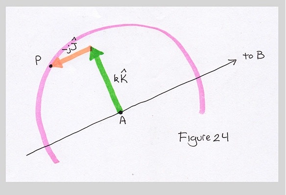
The expression for Q, out there at circle B, is just about the same, except we use the center B and radius $b$.
$$ j_b = b*\sin(\theta) \\ k_b = b*\cos(\theta) $$So then
$$ Q = B + (-j_b * \hat{J}) + (k_b * \hat{K}) $$There are built-in methods in almost every modern programming language to normalize, scale, add, and subtract vectors, so you don't have to do any of the math yourself. Processing has them, too. You do have to make the vectors in the first place, though. To make the un-normalized J, just subtract A from B:
$$ J = B-A $$Note that we have to follow this with a normalization step to get the vector $\hat{J}$ with length 1. To rotate this 90 degrees counter clockwise, we use the rotate-by-90 trick. Here's the recipe:
$$ K = (J_y, -J_x) $$If we already normalized $J$, then $K$ will be normalized, too. Otherwise well have to normalize $K$ as well.
Finally, you can find the other pair of points (let's call them P' and Q') just by flipping the direction of the scaled version of $\hat{K}$. We only need to multiply the scaling factors $k_a$ and $k_b$ by -1:
$$ P' = A + (-j_a * \hat{J}) + (-k_a * \hat{K}) \\ Q' = B + (-j_b * \hat{J}) + (-k_b * \hat{K}) \\ $$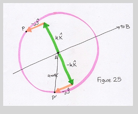
That does it! We now know how to find P, which unlocked Q, which made it easy to find P' and Q'. We put it all together as we saw in Figure 4, repeated here:
For completeness, here's the code in Processing. If you copy and paste this code into Processing, you'll get a new, random pair of circles once per second. To represent points and vectors I use PVectors (see the video "PVectors", Week 6, Group 7, Video 5).
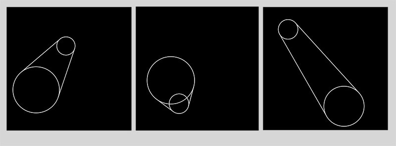
To start off, here are some pictures of the program running and joining up random pairs of circles.
PVector P, Q, Pp, Qp;  // the four points we compute

void setup() {
  size(800, 800);
  frameRate(1);  // cook up a new example every second
}

void draw() {
  background(0);
  float a = random(50, 100);       // pick a distance from the edge
  float b = a + random(50, 100);   // and a bigger one
  // find the two points A and B to serve as our circle's centers
  PVector A = new PVector(random(a,width-a), random(a,height-a));
  PVector B = new PVector(random(b,width-b), random(b,height-b));

  findBlend(A, B, a, b); // do the work to find our points

  stroke(255);
  noFill();
  strokeWeight(3);
  ellipse(A.x, A.y, 2*a, 2*a);   // draw circle A
  ellipse(B.x, B.y, 2*b, 2*b);   // draw circle A
  line(P.x, P.y, Q.x, Q.y);      // draw the line from P to Q
  line(Pp.x, Pp.y, Qp.x, Qp.y);  // draw the line from P' to Q'
}

// Given two circle centers and radii, set the globals P, Q, Pp, and Qp
void findBlend(PVector A, PVector B, float a, float b) {

  PVector J = B.get();   // J is B
  J.sub(A);              // now J is B-A
  J.normalize();         // now J has length 1

  PVector K = new PVector(J.y, -J.x);    // K is J rotated ccw by 90 degrees

  float d = dist(A.x, A.y, B.x, B.y);    // distance from A to B

  float theta = 0;                       // the angle by which we'll rotate our point
  if (d != 0) theta = asin((b-a)/d);     // if d isn't 0, compute theta
  float sintheta = sin(theta);           // save time by computing this just once
  float costheta = cos(theta);           // this too

  PVector sJ, sK;       // These hold scaled versions of J and K
  sJ = J.get();         // J is the normalized version of B-A
  sJ.mult(-a*sintheta); // scale it

  sK = K.get();         // K is the normalized perpendicular to J
  sK.mult(a*costheta);  // scale that

  P = A.get();          // To find P, start with A
  P.add(sJ);            //   add the scaled version of J
  P.add(sK);            //   and the scaled version of K

  Pp = A.get();         // To find Pp, start again with A
  Pp.add(sJ);           //   and add the scaled version of J
  Pp.sub(sK);           //   but now subtract the scaled K

  sJ = J.get();         // Repeat the above, but use circle
  sJ.mult(-b*sintheta); // radius b, and center B

  sK = K.get();
  sK.mult(b*costheta);

  Q = B.get();
  Q.add(sJ);
  Q.add(sK);

  Qp = B.get();
  Qp.add(sJ);
  Qp.sub(sK);
}
I hope this gave you a little encouragement to try solving geometry problems on your own. Give yourself time and lots of scratch paper, and follow your hunches. You'll get nowhere most of the time, but eventually something will usually pop out that's useful. Then you can clean it up and program it!