The AU Library:
Blending and Easing
Andrew Glassnerhttps://The Imaginary Institute
15 October 2014
andrew@imaginary-institute.com
https://www.imaginary-institute.com
http://www.glassner.com
@AndrewGlassner
Imaginary Institute Tech Note #4
Table of Contents
- Introduction
- Picturing Motion
- What to Look For
- The Curves
- The Linear Curve
- The Cubic Curve
- The Back Curve
- The Elastic Curve
- Hybrid Curves
- Using the Curves
- The Cosine Blend
- The S5() function
- The lerp() function
- Behind the Scenes
Introduction: Blends, Easing, Anticipation, and Elasticity
Animation is all about motion: where things go, and how they get there. So having good control over how things move is critical to making great-looking animation. We can think of motion as moving a shape from one place to another, but we can also think of it as blending the location of the shape over time.
Thinking of motion as blending is very powerful, because it let's us use simple tools to control lots of other things besides motion. For example, we can blend the setting suns color from yellow to orange, or blend a rabbits speed from slow to fast as it runs. We can also blend things in space, for example making them smaller and dimmer with distance.
Animators use a special kind of blending called easing , designed to make motion look organic and natural. When a creature that is at rest starts to move, it can't just instantly lurch into motion. Instead, it has to take some time to build up speed. And when it reaches its destination, it slows to a halt. This also looks great in computer animation.
Animators have other useful tricks for motion that we can borrow. When a character is about to do something important, you want to make sure your audience is looking at it. You can grab their attention in a very subtle but effective way: have your object make a small, fast motion. Humans are naturally drawn to small, quick motions, perhaps because catching the rustle of tall grass could save your life out on the savannah. A typical type of motion is to back up just a little, which can suggest that the character is anticipating the motion that is about to follow.
Sometimes a really fast-moving character can overshoot its target. Then it slows down and comes back, springing back and forth it goes until it finally comes to rest. This can look like the object is tied to its ending position on a rubber band, so this back-and-forth at the end is sometimes called elastic motion. It also tends to catch the eye.
This note describes a very simple-to-use library that lets you easily use all the effects we just discussed. The library does this by offering you a variety of blending curves. By the way, the word interpolation is sometimes used as a synonym for blending or easing.
Picturing Motion
In this section, well see pictures for the different basic types of motion. We'll also learn what to look for in these pictures to help us predict how things will move when we use these curves for animation. We'll also see the difference between motion paths (the shapes that objects trace out as they move) from motion curves (which tell us where we are on a motion path).
Motion curves almost always are drawn in the same way. To make these drawings as useful as possible, we don't refer at all to the geometry of the curve. All we know is that there is some path that takes our object from point A at the start to point B at the end. The job of the curve is to tell us where we are along that path at each moment in time.
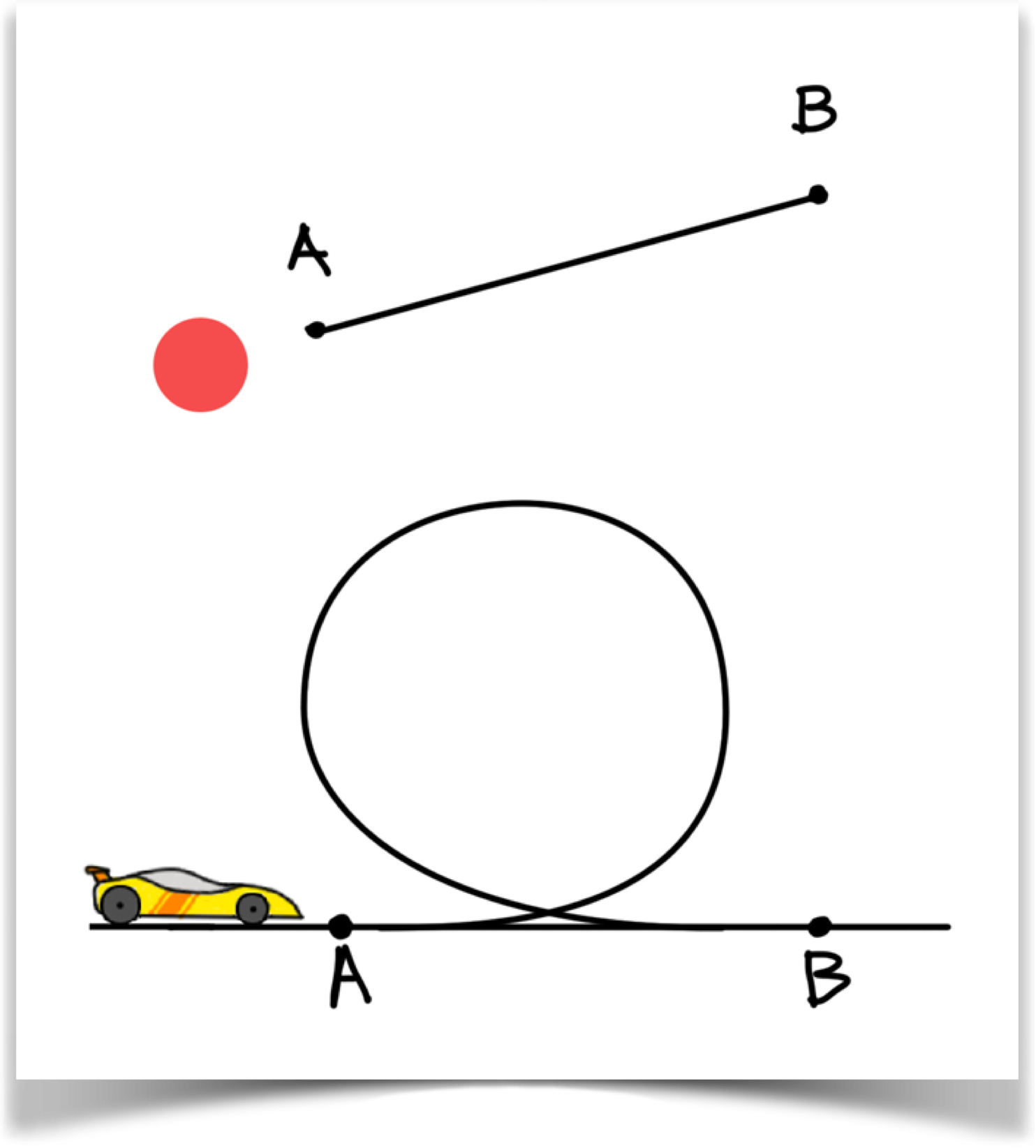
This is an important point, so let's see it in pictures. Suppose that you're animating a ball that moves from A to B along a straight line, as in the top parts of this figure:
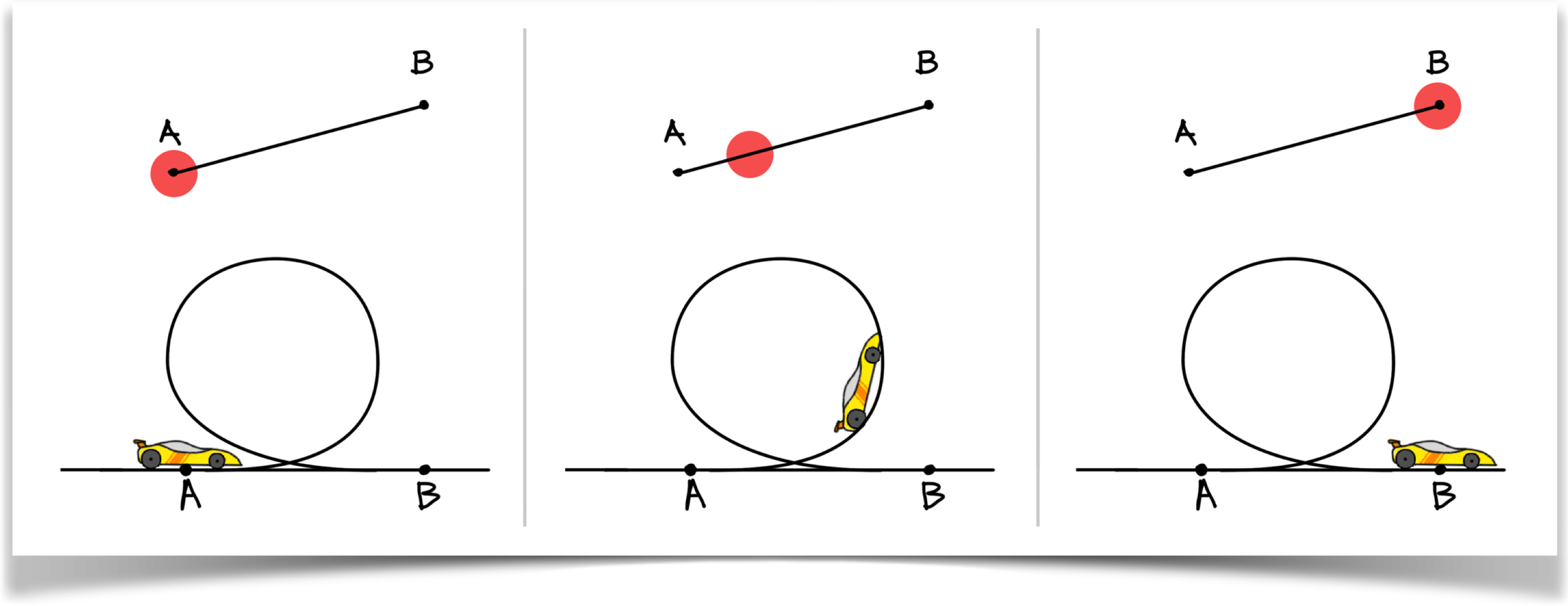
If at a given moment our motion curve tells us were 25% of the way along the path, then the circle will be on that line, 25% of the way from A to B. In the case of the race car, were also 25% of the way from A to B, but now were not on a straight line (in addition, the car has rotated, but ignore that for now - well come back to that later.).
Notice that for the race car, 25% along the path is not just 25% around the loop. There's some straight road after point A, and some more before point B, and we have to take both of these into account. Remember that when were told that the car is, say, 25% of the way from A to B, that is 25% of the total distance as traveled by the object from A to B. As with the race car, this is often not a straight line. We can use any shape of path we want, as long as we can put the object at any percentage along it.
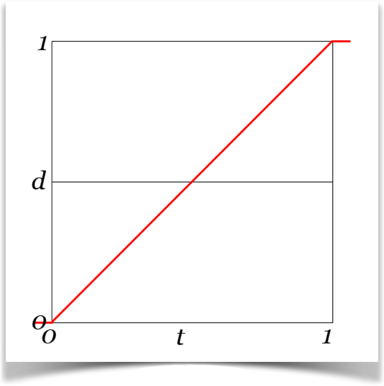
Motion curves are usually drawn in a standard form. We put time along the horizontal axis, running from left to right. Above each moment of time we place a single dot. The height of that dot tells us the percentage of our location along the motion path at that moment in time. When we space the dots closely enough, they join up to form a curve. Here's an example:
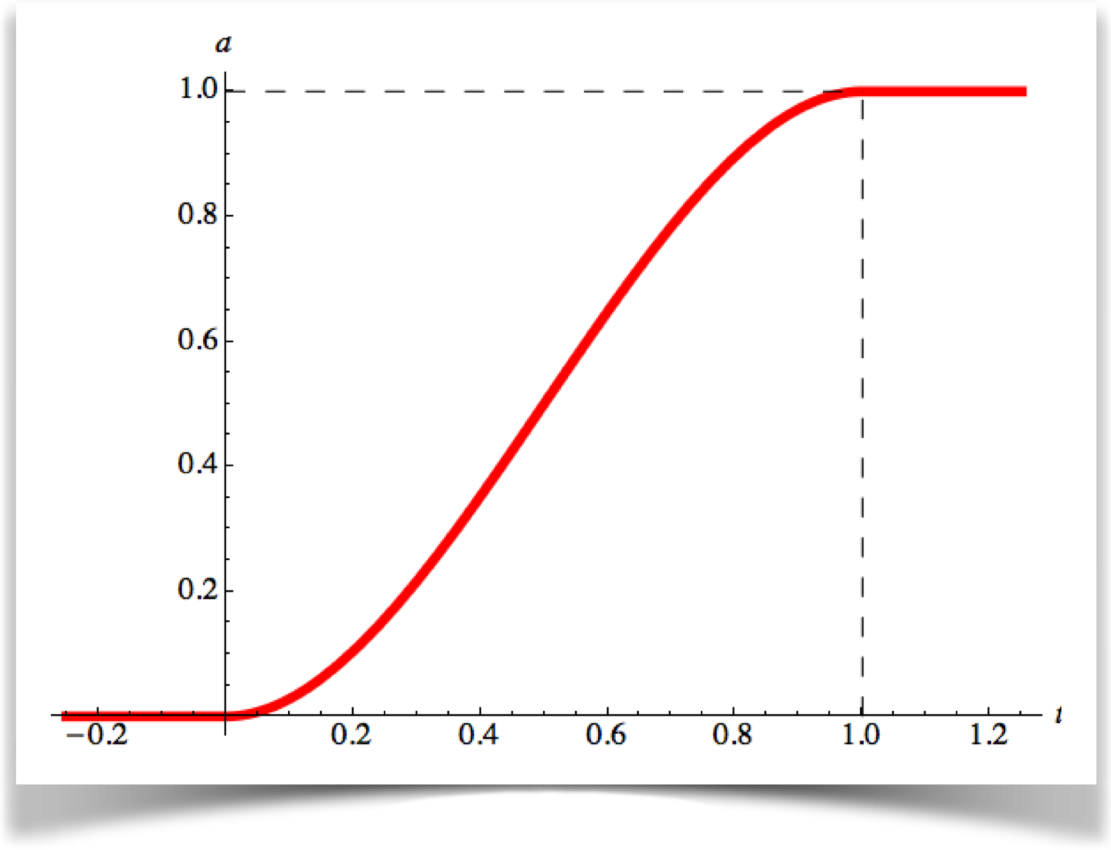
Reading the curve from left to right, we start at 0 (that is, the object is located at the starting point), we pick up speed, and by the time we reach time value 0.5 we're halfway along the path and moving quickly. Before long we slow down and settle into the final point, where we stay. So the curve just tells us the percentage of the way weve traveled; as we saw with the car and line, the path itself can have any shape at all.
Because we want these curves to apply with equal ease to animations of all sorts, we almost always set the drawings up the same way. The time axis, usually just written t , runs from 0 to 1. The height of the curve, which here I'll call d (for distance along the motion path), also runs from 0 to 1, representing the percentage weve traveled along the path. To read the graph, we plug in a value of t , and get back a value of d . For example, in this graph when t is about 0.65, the value of d is about 0.75, telling us that at time 0.65 were located at about 75% of the way along the motion path.
Of course, you'll usually want to use different ranges for both t and d. We'll see later that's very easy to do. In fact, these ranges of [0,1] for both t and d are used precisely because they make it easy to scale them to any other range.
In the next section well look at the curves supported by the library. To really understand those curves, and be able to envision what kind of motion theyll create, we need to be aware of a few particular things to look for. Let's look at those things now, and along the way well see some of the most important types of curves.
I'll start with the simplest curve. The object simply moves from the start to the end of the path at constant speed:
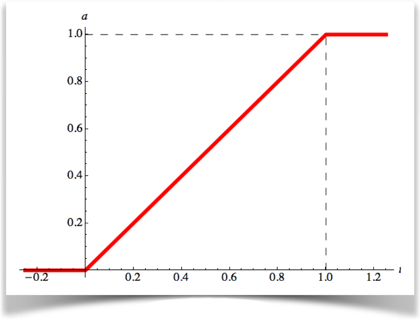
The plot is just a straight line, so we call this linear blending , or linear interpolation . We use this kind of blending all the time for little tasks that don't require the sort of natural-looking easing that well be looking at in a moment. Even though its a straight line, we call this a curve anyway (its just a really straight curve!).
You may notice that I've drawn values for the curve when t<0 and t>1. By convention, if you ask for the value of any curve for a time less than 0, you'll get back 0, and any time greater than 1 will return 1. Those little lines at the ends show just a piece of those ranges.
Let's try some nice easing, as described above: the ball starts off slowly, picks up speed, then gently slows down and comes to rest:
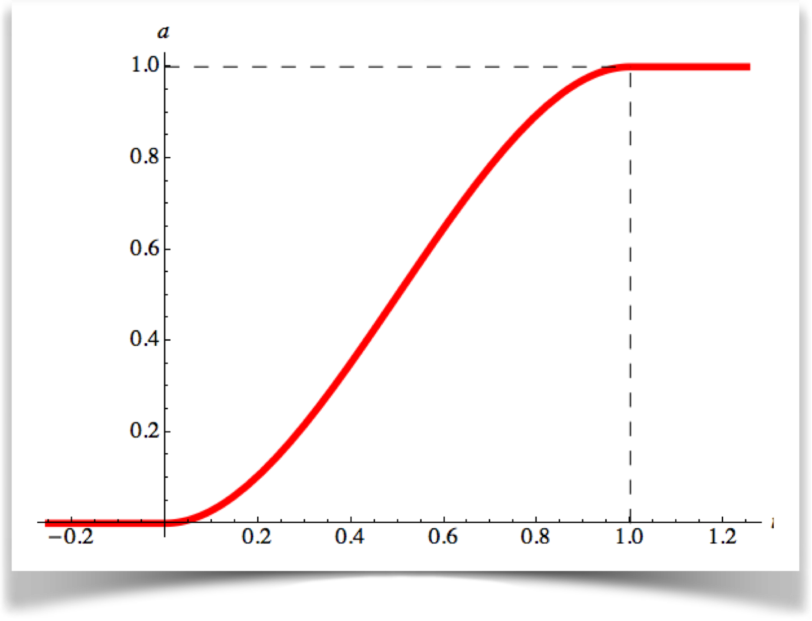
This is often called an S-curve (granted, the S is pretty stretched out). Its also frequently called the easing curve, since it's probably the most common curve used for that purpose. There are lots of subtle variations on this shape that give you slightly different motions, and we'll see some below, but they all have this distinctive shape.
The S-curve is incredibly popular for controlling almost anything moving on the screen. The gentle acceleration and deceleration feel organic and natural. Because its so useful, I wish that Processing had a little built-in function call that gives us the value of the S curve for any value of t. But there isn't, so my library provides one.
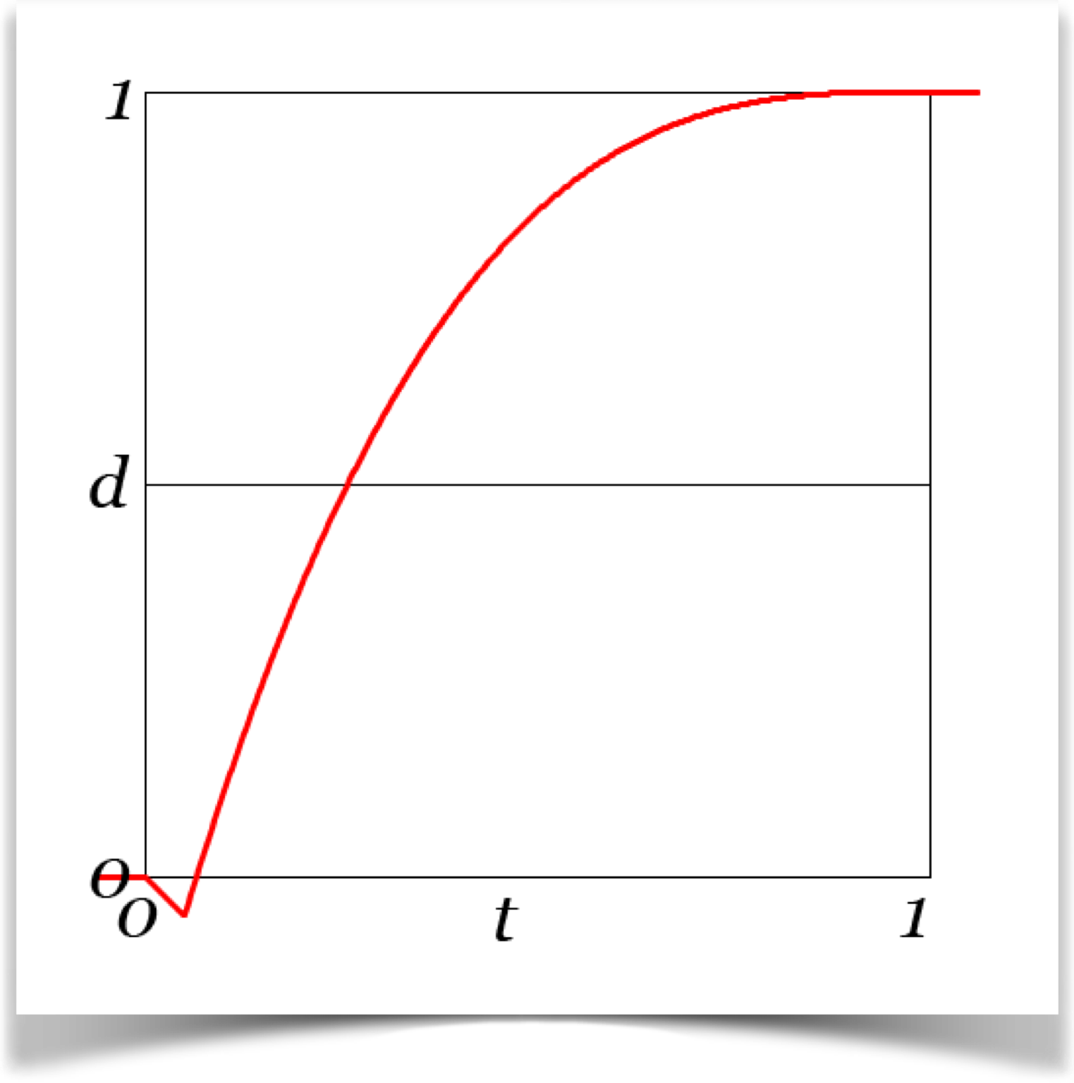
Let's see an example that combines anticipation with the linear curve:
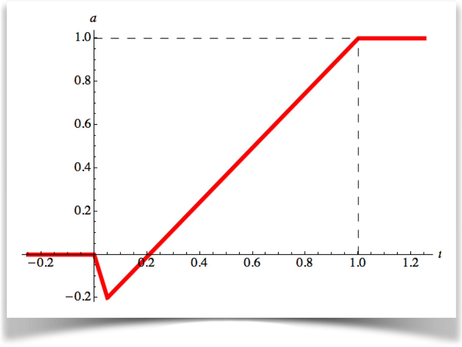
This curve has two important things you should be sure to notice.
First, unlike all our previous curves, the value d is not always between 0 and 1! For the first bit of the curve, d is in negative territory. For our application, that means the object is moving away from the ending point. Here are some examples of what that might look like for our car and line from above:
In the upper example, the dot has moved backwards along the line from A to B. In the lower example, the car has also moved backwards along the road. If the road was curved, the car would have followed that curved path, too (and wed have to rotate the car to make sure the wheels were still on the ground).
The second important thing about our anticipation curve is that the anticipation takes up some time. So the rest of the curve (in this case, the linear rise) gets modified a little bit. That means that the object will move just a little faster.
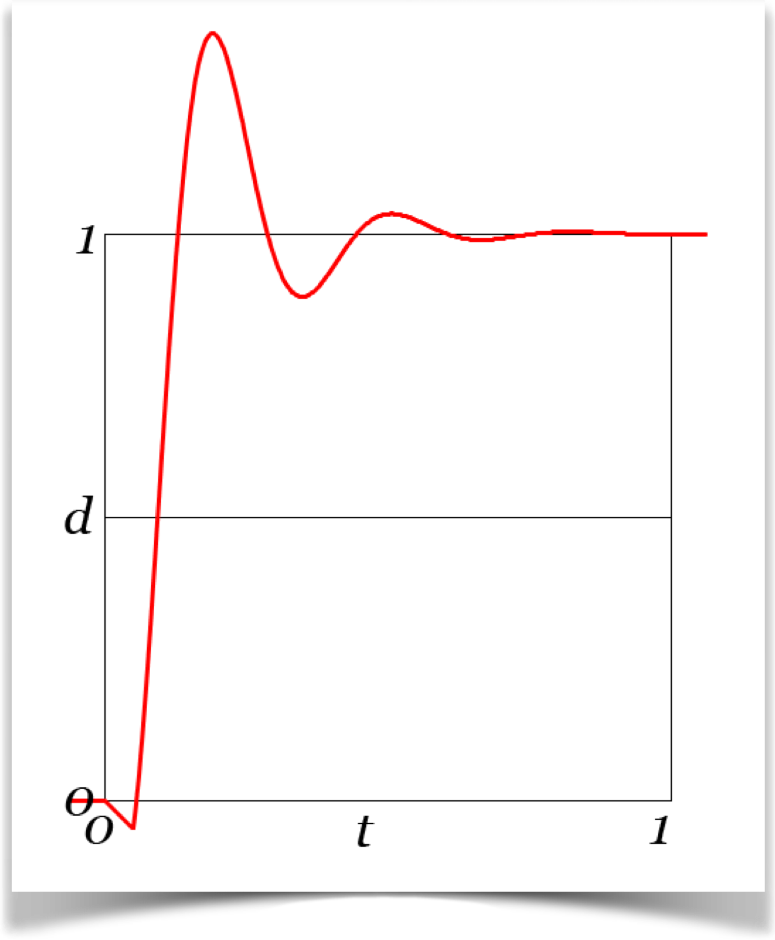
Moving on, let's look at elastic motion. Recall that this means overshooting the end point, then overcompensating by coming back, then overcompensating again, like a ball on a rubber band. Here's a look at this kind of action:
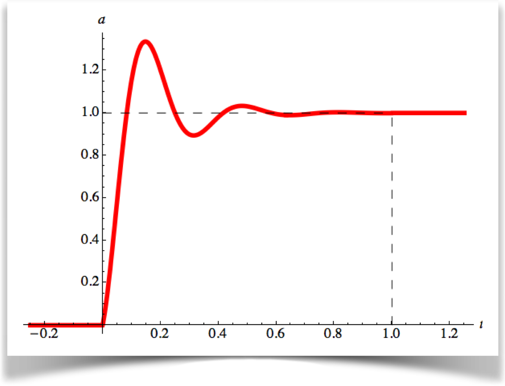
Here again, the curve returns values that are not between 0 and 1, but this time some values are greater than 1. When d >1, the curve is telling us to move to locations that are past the end point. Of course, its up to us to make sure we draw something sensible for these situations, no matter what the path is, just as we had to be able to handle values of d that were less than 0 in the anticipation curve.
If you can look at these motion curves pictures and see the motion of an object in your head, then you're home free. Everything else from here on is just fiddling with these curves, tweaking them and combining them in different ways.
What to Look For
There are a few things to look for in any motion graph.
First, it should begin at the start of the path, and end at the end. In numbers, this means it returns a value of d=0 for the input t=0 t and d=1 for the input t=1. All of the graphs in this library have this quality.
Second, it should be continuous. That is, it shouldnt abruptly jump from one value to another. This would look like the object had suddenly teleported along the path. The simple way to test for this is to ask yourself if you can draw the whole graph without lifting your pencil from the paper. If you can, its continuous. All of the graphs in this library are continuous.
The third thing to look for is whether or not the graph has any corners. Here, I'm using the word "corner" to mean any kind of sharp change in the direction of the graph. The linear graph in the figure has two corners: one at t=0 and another at t=1 The S-curve has no corners. The anticipation curve has corners at t=0, t=1, and about t=.1.
The reason corners are important is because they stand out visually, and grab the viewers attention. In fact, that's why I put them into the anticipation curve, because the whole point of the anticipation step is to grab the viewers eye. Its a powerful effect, and as I mentioned before, it should be used sparingly. You definitely don't want to be yanking the viewers eye all over your window as your animation progresses. So in general, you want to use curves that are nice and smooth, and only use curves with corners when you really need your audiences attention at that spot.
That's another reason the S-curve is is incredibly popular: not only does the motion gracefully accelerate and then decelerate, but there are no corners in the graph, so the motion produced by this curve looks natural and doesn't call attention to itself.
Sometimes people refer to corners by their mathematical description: a discontinuity in the derivative. Whatever you call it, your audience will look at it.
The Curves
The curves in the library all start at 0 when t=0 and end at 1 when t=1, and they are all continuous. What changes from one to the other is how they get there, and whether or not they have corners at their ends.
First, an acknowledgement. The curves in this library are mostly based on a package that Robert Penner created for Flash programmers, using a language called ActionScript. I don't know when he wrote that code, but I think it was in the 1980s. I've used Penner's names for his curves (though I've also added a few of my own). Though all my code is new, the underlying conceptual mathematics are the same. So if you're one of the many Flash animators who have used Penner's library, the curves in this library will be instantly familiar. Note that I didnt reproduce all of Penner's curves, but instead I picked the ones that I felt were the most useful.
In this section well look at each curve and discuss its key properties. In the next section, well see how to call the library to actually use these curves in practice.
Remember that for all curves, if t<0 we get back 0, and if t>1 t we get back 1. I'll include a little bit of those regions in each picture. I made these figures in Processing, using my library.
The Linear Curve
We'll start with the simplest curve: a straight line. Thus, we call it a linear curve, which is a bit of an oxymoron. This just produces a value of d that is equal to the value of t that goes in:
The Cubic Curve
This curve gets it name from the mathematical function that is used to define it: a cubic function. We can make three different curves by using that function at just the start (called the IN version), just the end (called the OUT version), or both ends (called the IN_OUT version). The IN_OUT version is precisely the very popular S-curve we saw in earlier, and is definitely the most commonly-used curve in the library.
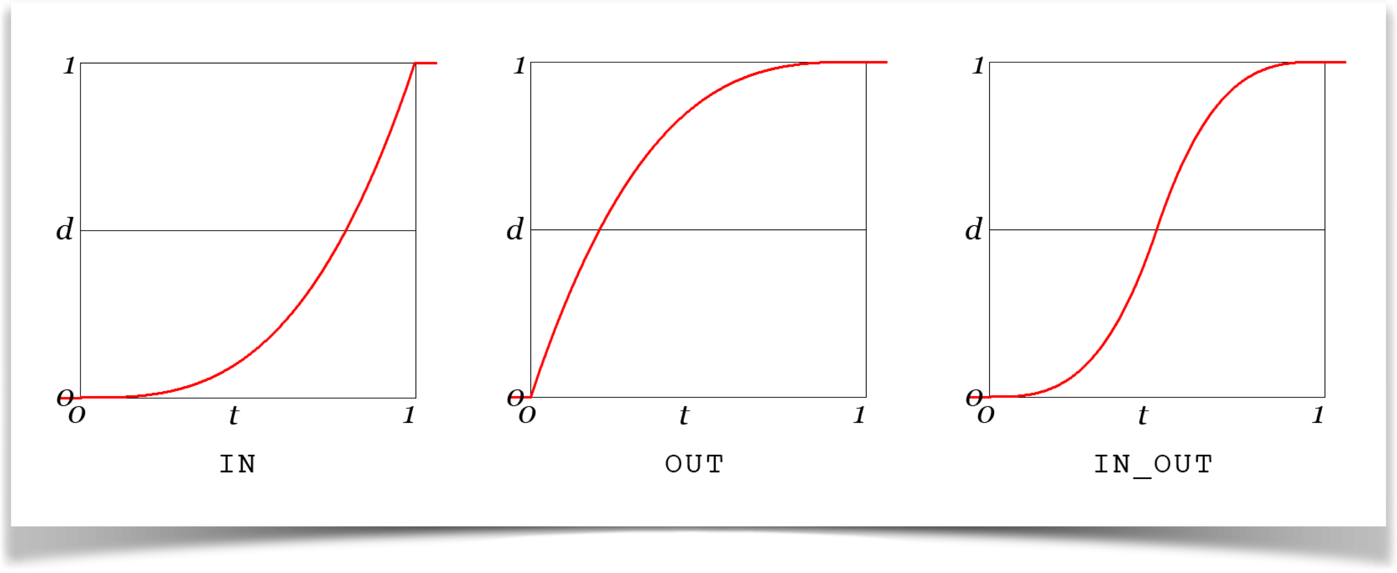
The IN version slowly accelerates, which looks great, but it freezes to a sudden halt at the ending location, which usually looks very un-natural. Plus, there's a corner there, which is eye-grabbing. When would we ever want such behavior?
You might use this curve when an object collides with another and instantly stops or even disappears. A soap bubble might use this curve, gradually rising from the moment its released until it reaches some height where it pops. More often, if your ending point is off-screen, then you don't really care how the object behaves out there, so coming to a sudden halt is no better or worse than anything else.
The same issues apply to the OUT version. You might use this if your starting position is off-screen (so nobody can see the sudden start), or for something like someone shooting a marble on a sandy playing field: the marble starts off suddenly moving fast, then slows down as it drags in the sand.
Its nice to have these around, but by a wide margin the most common cubic is the IN_OUT version. In fact, this and the linear curve are by far the most frequently-used curves in the library. The cubic S-curve is used all the time by programmers all over the world. Basically any time you are mixing or blending two things over time (or across the screen), applying the IN_OUT curve to the motion almost always makes everything just look better. Its definitely a contender for Animators Most Popular Curve.
The beauty of the cubic IN_OUT is that everything is smooth as can be. You start out at rest, then gradually pick up speed, then move quickly, and then gradually slow down before coming to a graceful rest. There are no corners. It looks organic and natural.
The Back Curve
The back curves get their name from the IN version, which seems to go backwards for a while before going forward. Literally, your object will start out by smoothly moving backwards , then smoothly will smoothly slow down and then head towards the ending spot, where it arrives while moving fast.
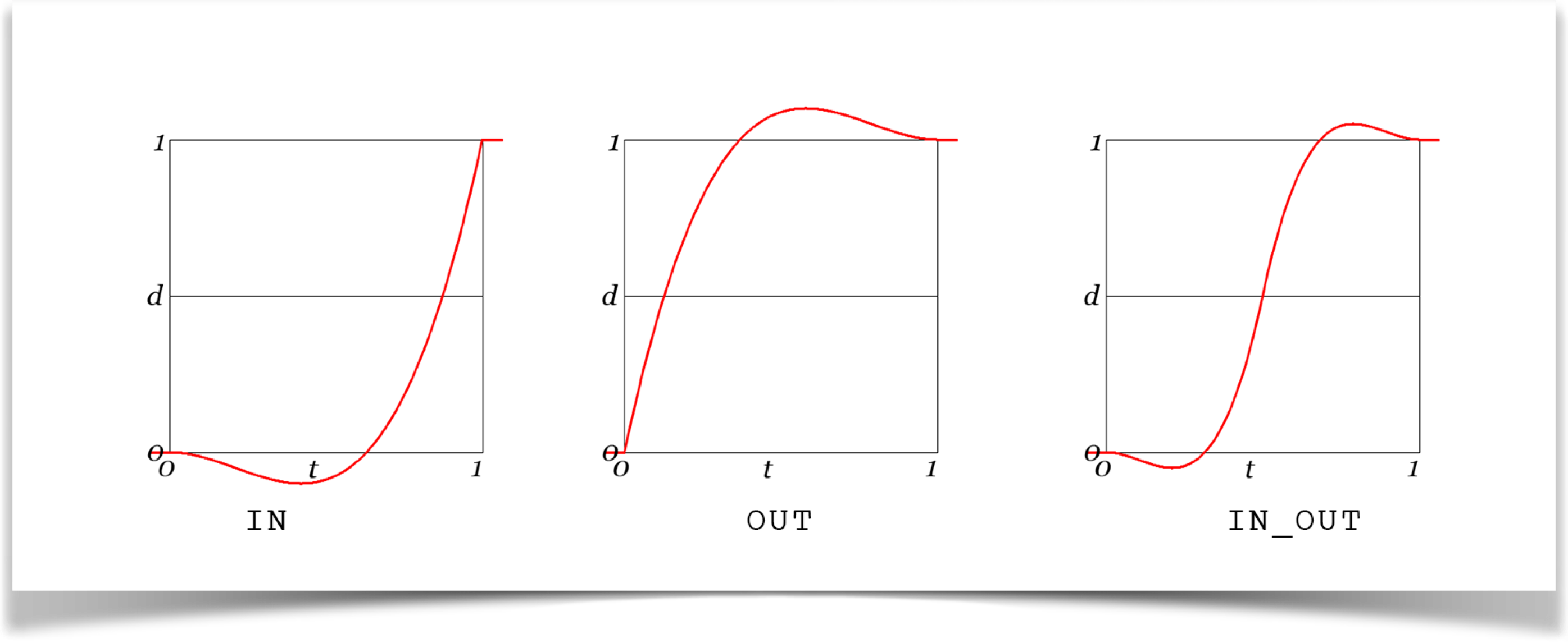
Note that this isn't going to be much good if you want anticipation. The requires a small, quick motion, and the backwards sweep of the back IN is just too big and slow. We'll see effective anticipation in a bit.
As you can see, the OUT version does the opposite of IN: you start out moving fast, overshoot the end position, and then slow down before coming back to rest at the ending point.
The IN_OUT version combines the two. This is nice and smooth at both ends, making it one of many variations on the ever-popular cubic S-Curve we saw above. As with the cubic, the IN and OUT versions each have a corner, while the IN_OUT does not.
If you look closely, you may notice that the IN_OUT version undershoots and overshoots by less than just the IN or OUT versions alone. In fact, it goes just half as far. The IN version drops down to -.1 before rising, and the OUT version rises up to 1.1 before dropping back down to 1. In other words, they undershoot and overshoot the range [0,1] by 10%. So when you set up a scene that uses these curves, make sure that you can reasonably use values from -1.1 to 1.1. The IN_OUT version goes outside the range [0,1] by half that amount, or 5% of the total range: the undershoot goes down to -0.05, and the overshoot goes up to 1.05. That's how Penner made his curves, and the combined weights of history and compatibility guided me to make my curves behave that way, too.
The Elastic Curve
Next, we consider the elastic curve, named because it looks like the object is on a piece of elastic tied to the end point of the path. We overshoot the end point, come back (but overshoot again), and bounce back and forth, a little less each time, before coming to a smooth stop.
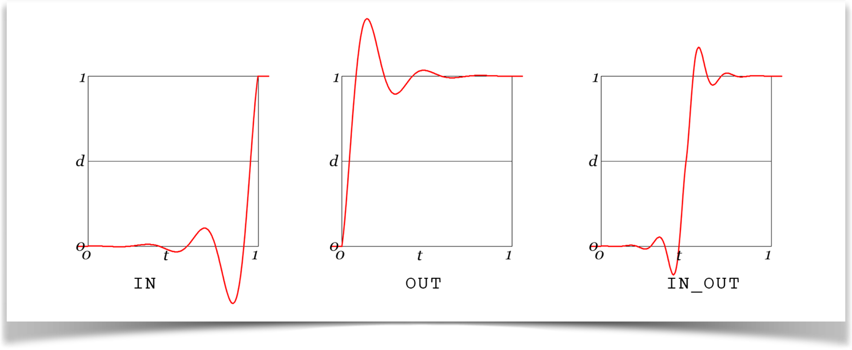
I just described the OUT version. Just for consistency, there's also an IN version, where the object starts at rest at the start point, then vibrates with more and more energy until it shoots for the end point.
The IN curve shoots down to -0.6, and the OUT curve pops up to 1.6. That is, IN has a range [-0.6, 1] and OUT has a range [0, 1.6]. As with the BACK curves, the IN_OUT version goes half as high, so its range is [-0.3, 1.3].
As before, the IN and OUT versions have corners, while the IN_OUT version does not.
Hybrid Curves
I've made a few hybrids of the above curves that I've found useful. Like the linear curve, these are one-offs: they don't have three variations.
These all use anticipation and/or elasticity. Recall that both of these qualities should be used sparingly. As a general rule, you should not yank your audiences gaze around more than you really need to, and you should never be directing your viewers attention to more than one place on the screen at a time.
Smooth forms of easing, like the S-curve, don't need to be used so carefully. Generally speaking, it rarely hurts to just apply smooth easing to everything that moves!
Cubic to Elastic
Objects on this curve start out slowly, overshoot, and then bounce to a rest. There are no corners.
Anticipate to Cubic
This curve includes anticipation: your object will make a small, sudden jump backwards, then move towards the end point where it comes to a gentle rest.
Note that the curve has two corners: one at t t=0, and another slightly later when it changes direction from moving backwards to forwards. I put those in there on purpose, because the whole point of the anticipation step is to grab the viewers eye. The short, fast motion of anticipation should get your audience to pay attention to this object, but the quick changes in motion created by the corners act as another visual magnet.
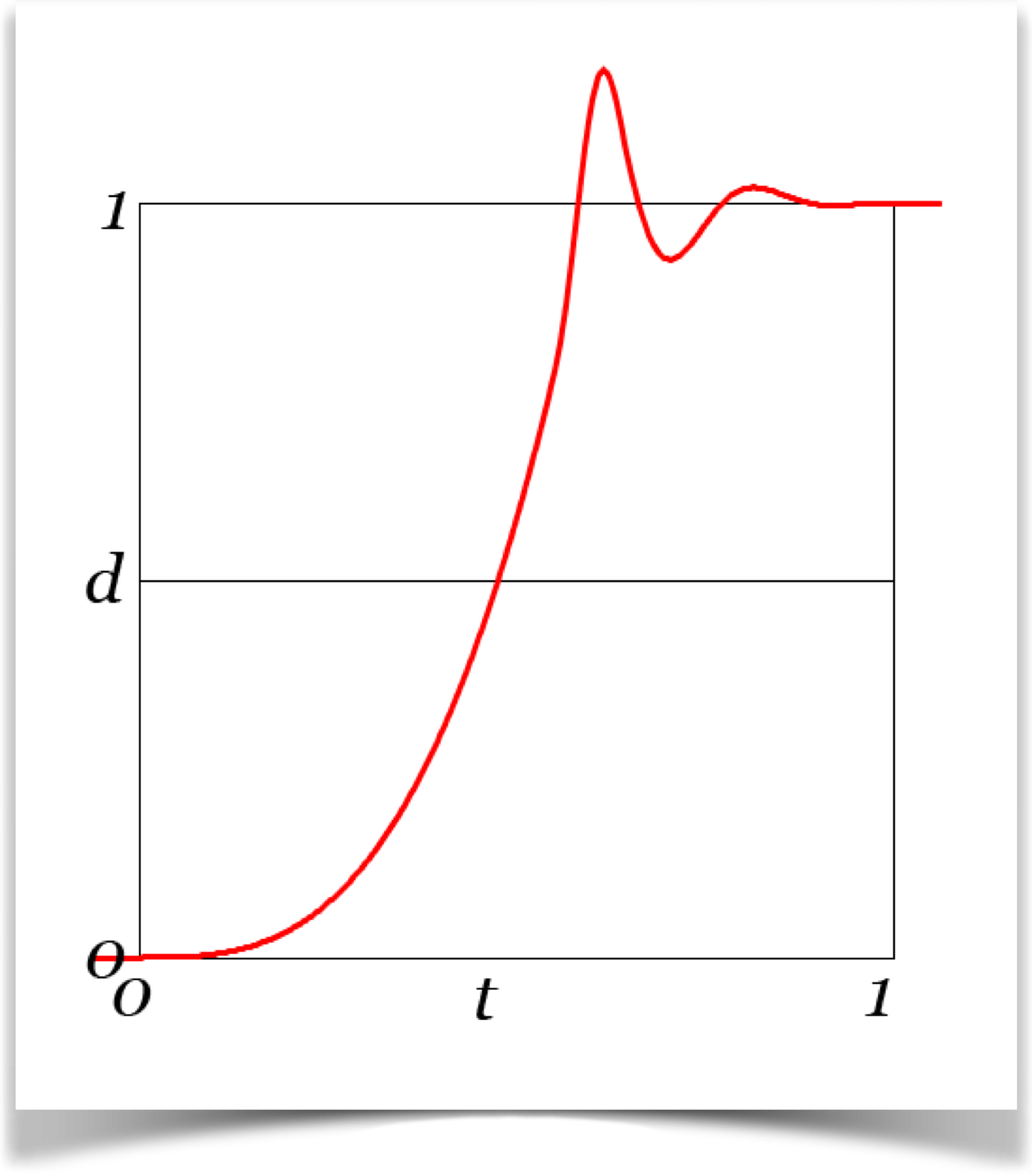
Anticipate to Elastic
This curve anticipates motion just like we saw in the last one, but instead of
coming to a smooth halt it bounces around the end point in the manner of the
elastic curves, and then comes to rest.
Using the Curves
The library is easy to use: there's only one function: ease(). You hand it a value telling it which curve you want (selected from the list below), and a value of t (a float from 0 to 1), and you get back a float that tells you the height of the curve for that t. Here's the call:
float AULib.ease(int curveNum, float t);And here's an example for using it to find the value of the INOUT cubic curve at time t=.3:
float d = AULib.ease(AULib.EASE_IN_OUT_CUBIC, 0.3);That's the whole thing. Values of t less than 0 will return 0, those greater than 1 return 1. In between, you get the curve.
Here's the list of curves, in the same order we covered them above.
| type | min | max | corner start | corner end |
|---|---|---|---|---|
| EASE_LINEAR | 0 | 1 | C | C |
| EASE_IN_CUBIC | 0 | 1 | - | C |
| EASE_OUT_CUBIC | 0 | 1 | C | - |
| EASE_IN_OUT_CUBIC | 0 | 1 | - | - |
| EASE_IN_BACK | -1.1 | 1 | - | C |
| EASE_OUT_BACK | 0 | 1.1 | C | - |
| EASE_IN_OUT_BACK | -0.05 | 1.05 | - | - |
| EASE_IN_ELASTIC | -0.6 | 1 | - | C |
| EASE_OUT_ELASTIC | 0 | 1.6 | C | - |
| EASE_IN_OUT_ELASTIC | -0..3 | 1.3 | - | - |
| EASE_CUBIC_ELASTIC | 0 | 1.3 | - | - |
| EASE_ANTICIPATE_CUBIC | -0.05 | 1 | C | - |
| EASE_ANTICIPATE_ELASTIC | -0.05 | 1.6 | C | - |
The second and third columns tell you the smallest and largest value you'll get back for that curve (rounded to two decimal places). Note that these arent the starting and ending values, which are always 0 and 1 respectively. Rather, these are the smallest and largest values across the entire curve.
The third and fourth columns remind you which curves have a corner at the start or end. Corners are marked with C. Remember that the anticipation curves also have a second corner soon after they get going.
All of our curves are defined for a time range from 0 to 1, and give back a value from 0 to 1. Let's now see how to use other ranges.
As a concrete example, suppose we want to move a circle from a point (30, 40) to a point (200, 250). The move should start at frame 50 and finish at frame 150. Furthermore, youd like the motion to look natural, so you'll use a cubic S curve.
First, we want to convert the frame number (given by the Processing variable frameCount ) into a value that is 0 at frame 50, and 1 at frame 150. The Processing function norm() will do just that:
int startFrame = 50;
int endFrame = 150;
float t01 = norm(frameCount, startFrame, endFrame);
Of course, you could put the numbers right into the call to norm() , but I usually use variables for these sorts of things, so I'll do that here (I use named variables so that I can easily find what to change if I come back to the program later, and want to fine-tune it).
The result of this call to norm() is exactly what we want. t01 will have the value 0 when frameCount has the value startFrame , and 1 at endFrame , and a value that smoothly rises from 0 to 1 in between (in fact, this is just a linear blend from 0 to 1!). When frameCount is less than startFrame , norm() will give us back a negative number. Similarly, when frameCount is greater than endFrame , norm() will give us back a number greater than 1. Remember that our curves are all defined to be 0 when t is negative, and 1 when t is greater than 1, so its perfectly fine to hand them the values of t01 computed by norm() .
Now we can just call our curve routine with this value of t :
float d = AULib.ease(AULib.EASE_IN_OUT_CUBIC, t01);
Remember that EASE_IN_OUT_CUBIC , like all the curves, returns values from 0 to 1. How do we use these to move our object?
Easy! We just blend the X coordinates and the Y coordinates separately, using d . We can use lerp() to blend them (again, a linear blend!).
float x = lerp(30, 200, d);
float y = lerp(40, 250, d);
Here I used numbers rather than variables, just for variety.
That's it! The result is that x and y will move from 30 to 200, and 40 to 250, respectively, following the motion of the cubic S curve. That is, a circle always drawn with its center at these values of (x,y) will start at rest, then slowly start to move, pick up speed, and then gracefully slow down before coming to rest at (200, 250).
Here's the whole program, soup to nuts. For variety, rather than providing the ending frame, I'll provide the duration of the move. The end frame is just the start frame plus the duration.
void setup() {
  size(300, 300);
}

void draw() {
  background(255, 240, 135);   // light yellow background
  fill(250, 70, 95);           // fill circle with a medium red
  float x0 = 30;               // starting x
  float y0 = 40;               // starting y
  float x1 = 200;              // ending x
  float y1 = 250;              // ending y
  int startFrame = 50;         // when we start moving
  int motionLength = 100;      // duration of move, in frames
  float t = norm(frameCount, startFrame, startFrame+motionLength);
  float d = AULib.ease(AULib.EASE_IN_OUT_CUBIC, t);
  float cx = lerp(x0, x1, d);  // blend x using the curve value
  float cy = lerp(y0, y1, d);  // blend y using the curve value
  ellipse(cx, cy, 40, 40);
}
If you want to have the circle anticipate a little bit at the start and slow down at the end, just use
float v = AULib.ease(AULib.ANTICIPATE_THEN_EASE, t);
If you want it to start slow and bounce at the end, use
float v = AULib.ease(AULib.EASE_SLOW_THEN_ELASTIC, t);
Of course, you can use any curve you want. that's all there is to it!
There's an important subtlety here that I want you to notice. Were using lerp() to blend the x and y values to position the circle. In other words, there are two blending steps going on. The first one takes the current time and returns a value from 0 to 1 that follows the smooth S curve: it starts slowly, picks up speed, then slows down as it reaches 1. Then we take that value and use it to control the calls to lerp() , which actually creates the blended value.
Now let's make a little change, and set the ball up so it bounces back and forth between these points forever. All we have to do is make sure we make the proper value of t .
Here's how I did it. I set a variable f to frameCount modulo twice the length of the motion. This gives us a number from 0 to (2*motionLength)-1 . If f is less than motionLength , I do nothing. If its greater, then were on the way back, and I do a subtraction so that f runs backwards from (motionLength-1) down to 0 .
void setup() {
  size(300, 300);
}

void draw() {
  background(255, 240, 135);   // light yellow background
  fill(250, 70, 95);           // fill circle with a medium red
  float x0 = 30;               // starting x
  float y0 = 40;               // starting y
  float x1 = 200;              // ending x
  float y1 = 250;              // ending y
  int motionLength = 100;      // frames from start to end
  int f = frameCount % (2*motionLength); // round trip
  if (f > motionLength) f = (2*motionLength) - f;
  float t = norm(f, 0, motionLength);
  float d= AULib.ease(AULib.EASE_IN_OUT_CUBIC, t);
  float cx = lerp(x0, x1, d);  // blend x using the curve value
  float cy = lerp(y0, y1, d);  // blend y using the curve value
  ellipse(cx, cy, 40, 40);
}
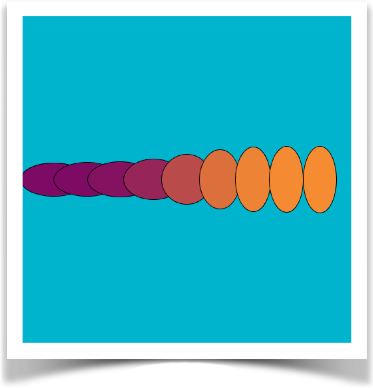
In these examples the parameter t was used for time. That's a common usage, but we can vary things in other ways, like based on their screen position. Suppose we want to draw a row of ellipses that change in their radii. Then t could just be the horizontal position of the ellipses center.
Here's an example. This program doesn't even need a draw() , since its doing no animation. I'll throw in some color blending just for fun:
void setup() {
  size(500, 500);
  float bigAxis = 100;                          // largest axis length
  float smallAxis = 50;                         // smallest axis length
  color leftColor = color(125, 10, 100);        // purple
  color rightColor = color(245, 140, 50);       // orange
  color backgroundColor = color(0, 180, 205);   // light blue
  background(backgroundColor);
  for (int x=50; x<=450; x+=50) {            // move right
    float t = norm(x, 50, 450);                 // turn position into [0,1]
    float v = AULib.ease(AULib.EASE_IN_OUT_CUBIC, t);
    float xaxis = lerp(bigAxis, smallAxis, v);  // blend the x axis
    float yaxis = lerp(smallAxis, bigAxis, v);  // blend the y axis
    fill(lerpColor(leftColor, rightColor, v));  // blend the color
    ellipse(x, 250, xaxis, yaxis);              // draw the ellipse
  }
}
And here's the result of the program:
Although I wrote my animation examples by counting frames, you might want to consider instead using millis() to find out how long your program has been running. This would be better for those times when you care more about how much time has elapsed than how many frames have been drawn.
There's one other thing to mention. Remember that I said the S-shaped cubic curve was the most popular of all? Just for convenience, it has its own little shortcuts. Just hand it one variable, the value of t :
v = AULib.cubicEase(t);
But this is so popular, it has a second shortcut: just the letter S, for S-shaped curve:
v = AULib.S(t);
I promised earlier to return to the rotating car. Aways remember that the library gives us a percentage traveled along the motion path. How we turn that into a picture is up to us. In the race car, if I want the wheels to stay on the track, my program would have to take the percentage, turn it into a position, and then rotate the car accordingly. Or suppose we were animating a nervous handyman climbing up a ladder. The library would give us a percentage along the ladder, and wed turn that into a position, and then draw more anxious shaking the higher he climbs.
The Cosine Blend
You may have heard of the "cosine blend". This comes from observing that if you take the first half of the cosine curve, flip it vertically, and scale it from 0 to 1, it looks just like a cubic S-curve:
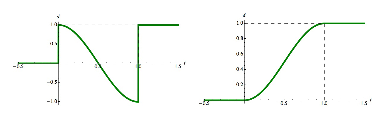
How close is this to the cubic S-curve? Let's draw them on top of each other:
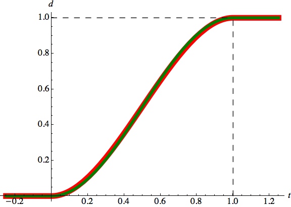
Wow. that's pretty close to a perfect match. I had to draw the cosine (in red) much thicker, just to see it under the cubic curve. In practice, youd never notice the difference between using one or the other.
But just for completeness, I've included a shortcut for the cosine S-curve. It just takes one parameter, t, like the shortcut for the cubic S-curve:
v = AULib.cosEase(t);
This complements the cubic version we saw above:
v = AULib.cubicEase(t);
v = AULib.S(t);
If the're so close, which one should you use?
To tell the truth, I've used the cosine version in most of my career, mainly because I didnt have to remember the coefficients for the cubic. But for this note, I wrote a little Processing sketch to compare them. I wrote a loop that called the cubic formula one hundred million times, and then found the average time for each call. I then replaced just the line evaluating the cubic with a line to evaluate the cosine curve.
On my computer (an early 2008 Mac Pro, with dual 2.8 GHz Quad-Core Xeon processors, running OSX 10.9.3 and Processing 2.2.1), the cosine version usually took about 70 times longer than the cubic!
So from now on I'll be using the cubic version, and I recommend that you do, too. that's why it has that super-short, one-letter shortcut name. But the cosine version is there just in case you need it.
If you want to replicate the experiment on your computer, I used this line for the cubic:
v = (t*t)*(3-(2*t));
and this line for the cosine:
v = (cos(PI*t)-1.)/-2.;
The S5() function
The cubicEase() function (also called S() for convenience) is pretty great. But if we tweak the mathematics a little bit, we can flatten it out a little more at the start and end. The resulting curve is called the S5() curve:
v = AULib.S5(t);
Here's the S5() curve in red, superimposed over the cubicEase() curve in green:
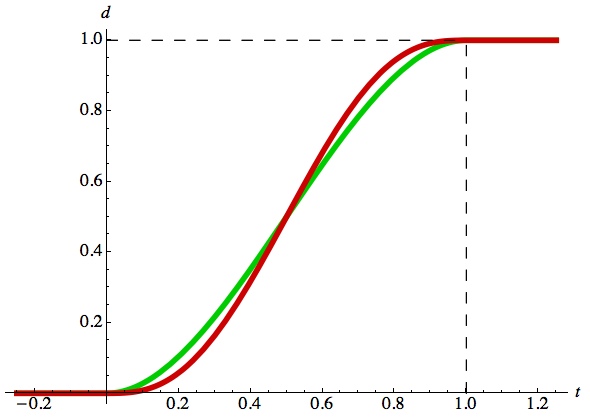
Note that flatter doesn't always mean better. I find that when used for motion, the S5() version seems to start late and finish early, because the motion at the ends is so small. But every now and then when you want this kind of feeling, its here for you.
The lerp() function
Let's pause to think about Processing's lerp() function, which we used above.
The function is doing a job very similar to our linear curve. In fact, its named for that task: the word lerp is a common contraction of "linear interpolation" (some people even spell it lirp, but usually we write it phonetically with an e). Processing's lerp() isn't intended for use just as a blending curve. Its a very general-purpose workhorse that gets used in a wide variety of ways. To keep it as general as possible, lerp() doesn't obey the convention of the blending curves, where values of t less than 0 or greater than 1 return 0 and 1, respectively. You can hand lerp() any value of t , even negative values, and you'll still get back a sensible blend.
To see what lerp() is doing, consider this call:
v = lerp(a, b, t);
where were blending from a to b , using t as our blending amount. When t =0 we get back the value of a , when t =1 we get back b , and of course values of t in between give us intermediate values between a and b . And, as I said, you can use any value of t and you'll still get a point along the line from a to b .
There are two equivalent, but distinct, ways to think about what lerp() is doing.
The first is that lerp() considers a to be the starting point, and over the course of the blend we add in more and more of (b-a) , the difference between the end and start points. We would write the implementation like this:
float lerp1(float a, float b, float t) return a + (t * (b-a));
Alternatively, we can think of lerp() as actually blending the two values. As t gets larger, we include less of a and more of b . We would write the implementation like this:
float lerp2(float a, float b, float t) return ((1-t)*a) + (t*b);
If you compare these, they of course give identical results. And since the're mathematically the same equation, technically there's no difference between these two versions. But I often find that one viewpoint or the other is a better conceptual fit with whatever I'm doing with lerp().
Behind the Scenes
In this section I'll describe the math and programming behind the curves. This is for folks who like to get under the hood. If you're not into this stuff, feel free to skip it. Nothing in this section is necessary for using the library.
The equations for these curves come from the ActionScript code originally written by Robert Penner (see http://www.robertpenner.com/easing/ for implementations in lots of different languages).
His library was pretty complicated, with a separate function call for each curve, each of which took 5 arguments. I'm pretty sure that's because he prioritized efficiency, so he squeezed all the norm() and lerp() calculations in my examples above together into a single routine. But computers are faster than in Ye Olden Days of early Flash programming, and I feel the simplicity and flexibility of having just one function call is worth an extremely tiny cost in time.
To make my curves completely compatible with his, I used his code to deduce the curve equations, and then I re-implemented them for this library. I'll go through them in the same order we used in Section 3.
Before I compute any curve, I test to see if were outside the range t =[0,1]. If we are, I don't even bother computing the curve value, I just return the right constant. The next two lines come before I evaluate any curve:
if (t<0) return 0;
if (t>1) return 1;
The Linear Curve
This is pretty easy. The formula is just
EASE_LINEAR: $f(t) = t$
The Cubic Curve
The cubic curve is simple:
EASE_CUBIC_IN: $f(t) = t^3$
To get the OUT version, just flip t around horizontally (use 1-t ) and vertically (subtract it from 1):
EASE_CUBIC_OUT: $f(t) = 1 - (1-t)^3$
That's the recipe for making the OUT version from the IN version for the cubic curves, bend curves, and elastic curves.
To make the IN_OUT version, just use the IN form from [0,.5] and the OUT form from [.5,1]. If you work it through, you'll see that this combination is continuous and smooth at the join for cubic, bend, and elastic curves. Here's the code:
// INOUT version of f(t)
if (t < .5) {
  float h0 = 2*t;
  return .5 * f(h0);
} else {
  float h1 = 1 * (1-t);
  return .5 + (.5 * (1 - f(h1)));
}
By the way, there's another way to make the IN_OUT version of the cubic. Rather than pasting together two half-curves, you can write the closed form of the S-shaped cubic directly. Its fun and easy to re-derive it from scratch, so let's do that.
We'll start with a general cubic as a function of t. There are four coefficients, which I'll name $a$ through $d$:
$$ f(t) = a t^3 + b t^2 + c t + d $$It will be useful to write down the derivative, which we can do just by looking. For convenience, I'll call the derivative $g(t)$:
$$ g(t) = 3 a t^2 + 2 b t + c $$We know we want the curve to have the value 0 at t=0 and 1 at t=1. We also want the curve to be flat at both ends, meaning the derivative is zero at those values of t. This gives us four constraints:
$$ \begin{align} {\rm 1:\ } f(0) &= 0 \\ {\rm 2:\ } f(1) &= 0 \\ {\rm 3:\ } g(0) &= 0 \\ {\rm 4:\ } g(1) &= 0 \end{align} $$Four constraints, four variables. We can find a, b, c, and c just by plugging things in. By plugging constraint 1 into $f(t)$, we find that $d=0$. Similarly, plugging 3 into $g(t)$ tells us that $c=0$. Were halfway there already!
Next, plug 2 into $f(t)$:
$$ 1 = a(1^3) + b(1^2) = a + b $$We got a simple result because we knew $c=0$ and $d=0$. Finally, plug 4 into $g(t)$:
$$ 0 = 3a(1^2) + 2b(1) = 3a + 2b $$These two equations are easy to solve. Rewrite $1=a+b$ as $b=1-a$, , then plug that value of $b$ into $0=3a+2b$:
$$ 0 = 3a + 2(1-a) = a+2 $$Which tells us $a= -2$. Popping that back into $1=a+b$ gives us $b=3$.
And there we have it. Our cubic is
$$ f(t) = -2 t^3 +3 t^2 $$That's exactly the same curve that we get from pasting together two half-cubics, but its nice and short and in closed form. In fact, this is the version I use in the shortcut for the S-shaped cubic. you'll see this formula over and over again, in countless programs, as people must re-derive and re-implement this dozens of times every day.
You can also think of this shape as a cubic Bezier curve with knots (0, 0, 1, 1). The explicit form here has an advantage over the Bezier (this is kind of technical, so don't worry if this means nothing to you): sampling a single-valued 2D Bezier curve in equal increments of t does not generally return equally-spaced points in x , but with the cubic you can easily supply equally-spaced values of t (representing x ) and avoid that problem.
The S5 Curve
The S() curve is a cubic polynomial. The S5() curve is a quintic (hence the 5 in the name):
$$ f(t) = 6 t^5 - 15 t^4 + 10 t^3 $$The Back Curve
The back curves are also cubics. The equation is
$$ f(t) = (1+g) t^3 - g t^2 $$where
$$ g = 1.70158 $$This is the closed form of a cubic Bezier with values $(0, 0, -g/3, 1)$.
This value of $g$ is specified in Penner's code. Unfortunately, he doesn't document where this number came from. But if you use this value and find the point of zero derivative, you find it at about $t=0.419753$. The value of $f(t)$ there is almost exactly $-0.1$, so I think this value of $g$ was chosen so that the curve would overshoot by just about exactly 10 percent. Why 10 percent? I don't know his thinking, but it seems to me that the exact choice for the amount of overshoot and undershoot is less important than simply knowing what that figure is. When you know the bounds of the curve, you can design your scene to make sensible use of all the values it produces. I'm guessing that Penner thought 10% looked good to his eye, and so he chose that as the target. The value of $g$ is simply the one that produces that result. Regardless of its origin, this is the value of $g$ that he uses, so for consistency with his curves I use it as well.
The Elastic Curve
The elastic curves are actually two little functions multiplied together.
The first is
$$ f_1(t) = \sin(6 \pi t) $$which produces three complete cycles of a sine wave. Conveniently, this curve begins and ends at 0 (though the derivatives at the start and finish are not 0).
The second curve is
$$ f_2(t) = 2^{10(t-1)} $$This is a scaling curve. When $t=0$, it has the value $2^{-10}$, or 1/1024, which is pretty close to 0. As $t$ moves closer to 1, the curve quickly rises up to 1 (remember that $2^0 = 1$). The elastic IN curve is just the product of these two:
$$ f(t) = \sin(6 \pi t) 2^{10(t-1)} $$I find this pretty clever. Its a nice and simple way to get the sine curve to start out small and get bigger. The only problem is that it isn't really 0 at $f(0)$, so in some circumstances (like if you're really zoomed in on the starting point), you could see a tiny jump at the start. Its close enough to 0 that I call it zero in our chart above, but in the back of my mind I know that 1/1024 isn't really 0. At the cost of a few more operations, we can get this to really run from 0 to 1:
float f1 = cos(6*PI*t);       // f1(t)
float f2 = pow(2, 10*(t-1));  // raw f2(t)
float minf2 = .000976563;     // 2^(-10) = 1/1024
float sclf2 = .999023;        // 1-minf2
float f2 = (f2-minf2)/sclf2;  // now f2(0)=1, f2(1)=0
return f1*f2;
As much as I like getting things right, I don't think this is really worth the effort. And his library doesn't do it this way, so I don't, either. But if you want to roll your own curve that really does start at 0, you can just copy and paste the code above.
Hybrid Curves
My hybrids are based on the equations above. To make the curves with anticipation, I start with a small backwards linear motion, and then tack on the usual curve, scaled and moved as necessary. The transitions from rest to the small motion, and then from the small motion to the main curve, are both sharp corners. that's fine, because the whole point of the anticipatory motion is to grab the viewers attention. If the little motion doesn't grab your viewers eye, the two corners should do it.
The curve blending the slow ease at the start with bouncing at the end was a little more tricky, because we have to somehow smoothly transition from a cubic to a decaying sine wave. The answer: a cubic S-curve! I just break up the interval of t from [0,1] into three sections: the cubic, the transition zone, and the decaying sine. In the blend section, I just use a very squished S-curve to blend the two shapes together smoothly.
The code is straightforward but lengthy. If you're interested, check out the source.
Resources
The equations for these curves come from the ActionScript code originally written by Robert Penner. See www.robertpenner.com/easing/. I didnt re-implement all of his curves, but instead chose just the ones I thought were most useful.
You can find pictures of these curves (though not my hybrids) at easings.net. A neat feature of this webpage is that if you hover over any of the curves, a little red arrow at the right of the curve will animate its vertical motion using that curve, so you can immediately see how it looks in practice.
Another nice description of basic blending (or interpolation) with animations is at http://sol.gfxile.net/interpolation/.
There are lots of implementations of Penners curves, and the're even in an existing Processing library named Ani. You can download it by following the library links at processing.org, or directly from its home page at http://www.looksgood.de/libraries/Ani/. Ani is very powerful, bit it has a different philosophy than the one adopted here.
The library, examples, documentation, and download links are all at the Imaginary Institutes resources page:
https://www.imaginary-institute.com/resources.php
To use it in a sketch, remember to include the library in your program by putting
import AULib.*;
at the top of your code. You can put it there by choosing Sketch>Import Library... and then choosing Andrew's Utilities, or you can type it yourself.
This document describes only one section of the AU library, which offers many other features. For an overview of the entire library, see Imaginary Institute Technical Note 3, The AU Library.
My thanks to Eric Haines, who read this document and offered many great suggestions that improved it.