Interpreting Alpha

Andrew Glassner
https://The Imaginary Institute
11 November 2014

andrew@imaginary-institute.com
https://www.imaginary-institute.com
http://www.glassner.com
@AndrewGlassner

Imaginary Institute Tech Note #10

Introduction

The idea of "alpha" has been a part of computer graphics for over three decades, since it was presented in the classic paper on image compositing [PorterDuff84].

The alpha idea been used to composite billions of pixels (if not more) to create images for print, video, film, and probalby every other application of computer graphics. The concept of alpha as part of a pixel's color is firmly embedded in our psyches and our code.

Alpha is obviously incredibly useful for compositing images, but what does it really represent? This memo will explore that question and try to provide a complete answer.

The graphics literature can seem to be hard to nail down on this issue. In their paper, Porter and Duff sometimes consider alpha to represent the opacity of a completely covered pixel:

If $\alpha_A$ and $\alpha_B$ represent the opaqueness of semi-transparent object which fully cover the pixel, the computation is well known.

At other times, they consider it to be the area of a pixel that is covered by a colored fragment within it (that area is called the coverage):

If $\alpha_A$ and $\alpha_B$ represent subpixel areas covered by opaque geometric objects, the overlap objects within the pixel is quite arbitrary.

The authors switch interpretations based on whatever is most useful at each moment in their discussion.

Porter and Duff are not alone in this. In a memo on the subject [Smith85], Smith states,

"There are two ways to think of the alpha of a pixel. As is usual in computer graphics, one interpretation comes from the geometry half of the world and the other from the imaging half. Geometers think of "pixels" as geometrical areas intersected by geometrical objects. For them, alpha is the percentage coverage of a pixel by a geometrical object. Imagers think of pixels as point samples of a continuum. For them, alpha is the opacity at each sample. In the end, it is the imaging model that dominates, because a geometric picture must be reduced to point samples to display - it must be rendered. Thus, during rendering coverage is always converted to opacity, and all geometry is lost. The Porter-Duff matting algebra that underlies what we present here is based on a model that is easiest to understand by alternating between the two conceptions."

So once again, alpha seems to be either coverage or opacity, depending on one's needs.

Finally, Blinn [Blinn94] says,

"The $\alpha$ value ... goes by various names: coverage amount, opacity, or simply alpha... I'm going to call it opacity for now. If it's 0, the new pixel is transparent and does not affect the frame buffer. If it's 1, the new pixel is opaque and completely replaces the current frame buffer color."

So Porter and Duff, Smith, and Blinn all treat alpha as a fluid concept, sometimes referring to opacity and sometimes referring to coverage, selecting the interpretation that seems most convenient at any given time.

A reader could be forgiven for finding this confusing. Coverage is a description of area, and opacity is a property of a color. It seems unlikely that a single number can mean either of these things depending on someone's momentary preference.

[Smith85] asserts that during rendering all geometry is lost, and only opacity remains. Must that be so? What if we don't throw away the geometry, but instead preserve it in the same way that we preserve opacity?

In this note, I'll do just that, and retain both opacity and coverage independently as we work through the compositing process. We'll find that the traditional equation for computing the new alpha after compositing emerges after the algebraic terms cancel one another out. But along the way we'll develop a better appreciation for what "alpha" is, and why it apparently can be be interpreted with such flexibility.

Pre-multiplying

Closely involved in any discussion of compositing is the idea of pre-multiplication.

In pre-multiplication, we store a color's components (typically red, green, and blue) already multiplied by alpha. For example, suppose we have a fragment with RGBA = $(1, .5, .25, .5)$ (in this document, all color values, opacity values, and coverage values will be in the range $[0,1]$). We could save that in pre-multiplied form as $(.5, .25, .125, .5)$. Note that the alpha value is unchanged, while the R, G, and B values get multiplied by alpha. [Blinn94] offers multiple situations where using pre-multiplied colors results in algorithms that are faster or easier to program. Here we'll look at two issues in particular: efficiency, and transparent pixels. Both of these issues are most easily discussed in terms of $over$, the most common compositing operation.

Before we see that, let's agree on notation. I'll write $A_c$ for any color component of a fragment of object $A$. Then this can typically be red, green, or blue. Since all components get treated in the same way, and independently of one another, we can focus on just one at a time. If you prefer, think of $A_c$ as a grayscale value. I'll write $A_\alpha$ for the alpha value of the fragment (for now, interpret that however you usually like to think of alpha). So we could write the color and alpha together as $(A_c, A_\alpha)$.

If we multiply the color by alpha before storing it, then we'd write $(A_\alpha A_c, A_\alpha)$. In this document, I'll use a lower-case italic letter to indicate a pre-multiplied value. Thus we'd write this as $(a_c, A_\alpha)$. Note that the alpha value $A_\alpha$ isn't itself pre-multiplied, so it gets a capital letter.

I'll refer to color values like $A_c$ that are not pre-multiplied as raw or straight colors (some people refer to pre-multiplied colors as associated and their non-pre-multiplied versions as unassociated).

With this notation, suppose we have two images $A$ and $B$. I'll use the same letters to refer to individual pixels of those images. I'd like to compose a pixel from $A$ over one from $B$. If they're not pre-multiplied, we can write this by adding the color of $A$ (multiplied by its alpha) and the color of $B$ (multiplied by its alpha), though because $A$ has an alpha of $A_\alpha$, it blocks $A_\alpha$ of $B$, so only $1 - A_\alpha$ of $B$ survives:

$$ C_c = A_\alpha A_c + (1 - A_\alpha) B_\alpha B_c \;\;\;\;\;\;\;\; (\rm{Eq.\;} 1) $$

This equation is actually not quite right; we'll return to it below. Taking it at face value for the moment, we need to do less work if the colors are pre-multiplied:

$$ c_c = a_c + (1-A_\alpha) b_c \;\;\;\;\;\;\;\; (\rm{Eq.\;} 2) $$

Note that the result is a lower-case $c_c$, since it's in pre-multiplied form as well. Equation 2 is the famous, standard equation for the over operation, which combines two pre-multiplied images.

Comparing Equations 1 and 2, we can see that the first reason for using pre-multiplication is efficiency. If we have many layers in our images, then we could easily be doing the over operation many millions of times per frame. The faster, pre-multiplied version in Equation 2 can save us a few multiplication operations at every pixel, which can add up to a lot of time.

The second advantage comes from noticing that in Equation 2, the alpha value for fragment $A$ is not applied to $A$, and the alpha value for $B$ doesn't even appear. That lets us do some interesting things by creating arbitrary combinations of $A_c$ and $A_\alpha$. For example, suppose you want to create a layer consisting of a single blue disk on a transparent background. Pixels that are entirely within the disk have a color of blue and an alpha of 1. Pixels that are entirely outside the disk have an alpha of zero. But what color do those uncovered pixels have?

The question is moot, because if a pixel is completely transparent, it doesn't matter what color it has. A common choice is to save the pixel color as transparent black, with pre-multiplied values $(0, 0)$ (in RGB, this would be $(0, 0, 0, 0)$). This is actually a bit of a misnomer, because it's not really black at all: it's completely transparent. But since $0$ is a grayscale black (and $(0,0,0)$ is RGB black), the name makes sense. Setting $A$ to transparent black and plugging it into Equation 2, we get:

$$ c_c = b_c $$

So if we compose a transparent black pixel on top of anything else, it makes no contribution. That is, it's transparent, as we intended. What if $B$ is the transparent black pixel?

$$ c_c = a_c $$

Again, thins work out nicely. Composing anything over transparent black just gives us back the new value.

Here comes the cool part. Suppose we make "transparent red" by setting the pre-multiplied RGB value of a pixel to $(1,0,0,0)$. I call a color like this (and transparent black, and any other color with an alpha of 0) a synthetic color, because it can't arise from any "natural" rendering process. For example, suppose that in a 2D painting program you set the color to $(1,0,0,0)$ and started to paint. The transparency of 0 means you'd have no effect on the underlying image. The only way to get a color like $(1,0,0,0)$ into a pixel is to write those components in there directly.

When we use the RGBA value $(1,0,0,0)$ for $A$ in Equation 2 (where I'll write subscripts $r, g, b$ to refer to the color channels), we get

$$ \begin{align} c_r &= a_r + b_r \\ c_g &= b_g \\ c_b &= b_b \end{align} $$

In other words, the red part of $A$ gets added in to the final color, but because $A_\alpha = 0$, the color of $b$ is not diminished at all. It's often useful to think of pixel filled with a synthetic color as a "glowing" pixel, one we might associate with a lens flare or the halo around a bright light or spark. It's color, but there's no opacity to it. It just adds its color in to the pixel below it. This effect is a result of how Equation 2 is structured.

We've seen two reasons to like the idea of storing color in pre-multiplied form: efficiency, and exploiting the idiosyncracies of the over equation to allow us to make synthetic colors, and from them, transparent pixels and glowing pixels.

Computing Composite Alpha

Suppose we want to use traditional alpha blending to stack up four images: $A$, $B$, $C$, and $D$. And suppose the most convenient way for us to compute these is to first form $F = A \text{ over } B$, and then form $G = C \text{ over } D$, and then put the two intermediates together to make $H = F \text{ over } G$. Then while computing $F$ we need to find not just the new color for each pixel, but a new alpha, so we can use it in the next stage when finding $H$.

[PorterDuff84] doesn't offer a formula for computing this new alpha. Both [Smith85] and [Blinn94] provide this expression for the composite of $A {\rm \;over\;} B$ (shown here in our notation):

$$ F_\alpha = A_\alpha + (1-A_\alpha) B_\alpha \;\;\;\;\;\;\;\; (\rm{Eq.\;} 3) $$

As usual, we write all the alpha values involved with capital letters, since they are not pre-multiplied by anything.

There's a lot to like about this formula: it's simple, it's satisfyingly similar to Equation 2, and thinking it through it makes intuitive sense. The formula is derived in [Blinn94] by working through the algebra of the over operator. In order to make that operation associative (which is very desirable), then this is the necessary expression. But that doesn't provide us with an intuitive interpretation of alpha. In other words, we know how to compute it, but we don't know how to interpret it.

In this document we'll re-derive this formula by carefully and independently tracking coverage and opacity. It turns out that Equation 3 indeed emerges at the end, and along the way we'll discover how to interpret the meaning of alpha.

Blending

Another important idea is blending. Suppose you have two scalar values, $p$ and $q$, and you want to mix some of each to produce a result $r$. One way to go is to multiply each of the inputs by a weighting factor. Whichever gets more weight will dominate in the output. For example, we could weight $p$ with $w_p$ and $q$ with $w_q$ to make

$$ r = w_p p + w_q q $$

There's a problem with this $r$, though: it incorporates the weights into the result, rather than just the values we're blending. To see this, suppose $p=.25$ and $q=.75$ and we want to combine them in the ratio $p:q = 2:1$. Then we can set $w_p=2$ and $w_q=1$ and get:

$$ r = (2 * .25) + (1 * .75) = 1.25 $$

On the other hand, I could choose weights $w_p=20$ and $w_q=10$. They're still combining the values in the same ratio, but the result is different:

$$ r = (20 * .25) + (10 * .75) = 12.5 $$

We would like to have a result that doesn't depend on the arbitrary values of $w_p$ and $w_q$, but only on their ratio, so that mixing the same ratio of $p$ and $q$ always gives the same result.

Of course, you're way ahead of me. To remove the influence of the weights, we need to divide the result by their sum:

$$ \frac{(2 * .25) + (1 * .75)}{2+1} = 4/9 = \frac{(20 * .25) + (10 * .75)}{20+10} $$

This is important to remember any time we're blending together values by weighting and summing them. To remove the effect of the weights, we must divide by their sum. We will use this fact below to keep our book-keeping straight as we track opacity through the composition operation.

But wait! We do linear interpolation all the time, using a formula like this:

$$ r = t p + (1-t) q $$

Why don't we divide by the sum of the weights? Easy: $t + (1-t) = 1$, so there's no need. As long as the weights sum to 1, we don't have to divide through by them. This is one reason people often normalize their weights, or make sure they add up to 1, before using them for blending.

But wait one more second. In Equation 2, the coefficients, or weights, on the colors are $1$ and $1-A_\alpha$. Shouldn't we be dividing the final color by $1+(1-A_\alpha)$? No, and that's part of the beauty of Equation 2. In this case, we want the weights to be included, because then the result is pre-multiplied. That is, the result includes the weights. That's why I wrote the left hand side in lower case. The standard over formula in Equation 2 gives us pre-multiplied results from pre-multiplied inputs because we don't normalize the result. This is a great deal: we save some calculations and we get a more useful result.

In Pre-Multiplying section, I said that Equation 1 wasn't "quite right". What's wrong with it? Of course, we're not normalizing the result. We're combining the colors $A_c$ and $B_c$ by using $A_\alpha$ and $(1-A_\alpha)B_\alpha$ as the weights. The results are pre-multiplied, and should have been written with a lower-case letter. The proper version of Equation 1 is

$$ C_c = \frac{A_\alpha A_c + (1 - A_\alpha) B_\alpha B_c}{A_\alpha + (1-A_\alpha)B_\alpha} \;\;\;\;\;\;\;\; (\rm{Eq.\;} 4) $$

We can see now that the pre-multiplied version of Equation 2 is even more efficient that we thought!

Opacity and Coverage

Let's set aside the idea of alpha for a moment, and instead make sure that we've got a good handle on distinguishing opacity and coverage.

Consider Figure 1, which shows a partly transparent orange ellipse over a transparent background (represented by the classic white-and-gray checkerboard). In this layer, think of every pixel starting as fully transparent (with a color such as transparent black), and then the ellipse gets rendered.

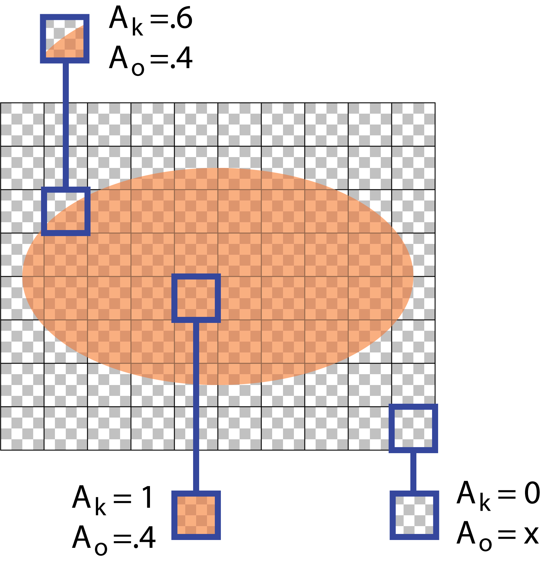
I've called out three pixels: one in the middle of the ellipse, one outside the ellipse, and one straddling an edge.

I'm going to associate two numbers with each pixel: coverage, written $A_k$, and opacity, written $A_o$. To understand these numbers, think of each pixel as containing a fragment. That's just a little piece of an object (in this case, the ellipse) clipped to the pixel's boundaries.

The pixel's coverage is nothing more than the fraction of the pixel that is occupied by the fragment.

The pixel's opacity is the opacity of that fragment.

This is important: neither of these are alpha. We're not thinking about alpha now, just area and opacity values, and each pixel simply inherits them from its fragment (later we'll see how these values change when we compose images and have multiple fragments per pixel. For now, there's just one fragment).

In Figure 1, the ellipse has opacity of $.4$ (that is, it blocks 40% of the color behind it, or, equivalently, allows 60% of that color to pass through).

The pixel in the center of the ellipse is fully covered, so $A_k=1$, and the fragment inside has the opacity of the ellipse, so $A_o=.4$. The pixel in the upper-left is about 60% covered by the ellipse, so $A_k=.6$, and the opacity of the fragment inside that pixel is again the opacity of the ellipse, so $A_o=.4$. The pixel in the lower-right that is outside the ellipse is not covered at all, so $A_k=0$. The opacity value $A_o$ is moot, since there's no fragment from which to derive an opacity value. I marked this $A_o$ with an x to indicate "don't know" or "don't care". In practice, we'd probably just set this to 0.

Consider now Figure 2, where the ellipse is fully opaque. I've called out the same three pixels.

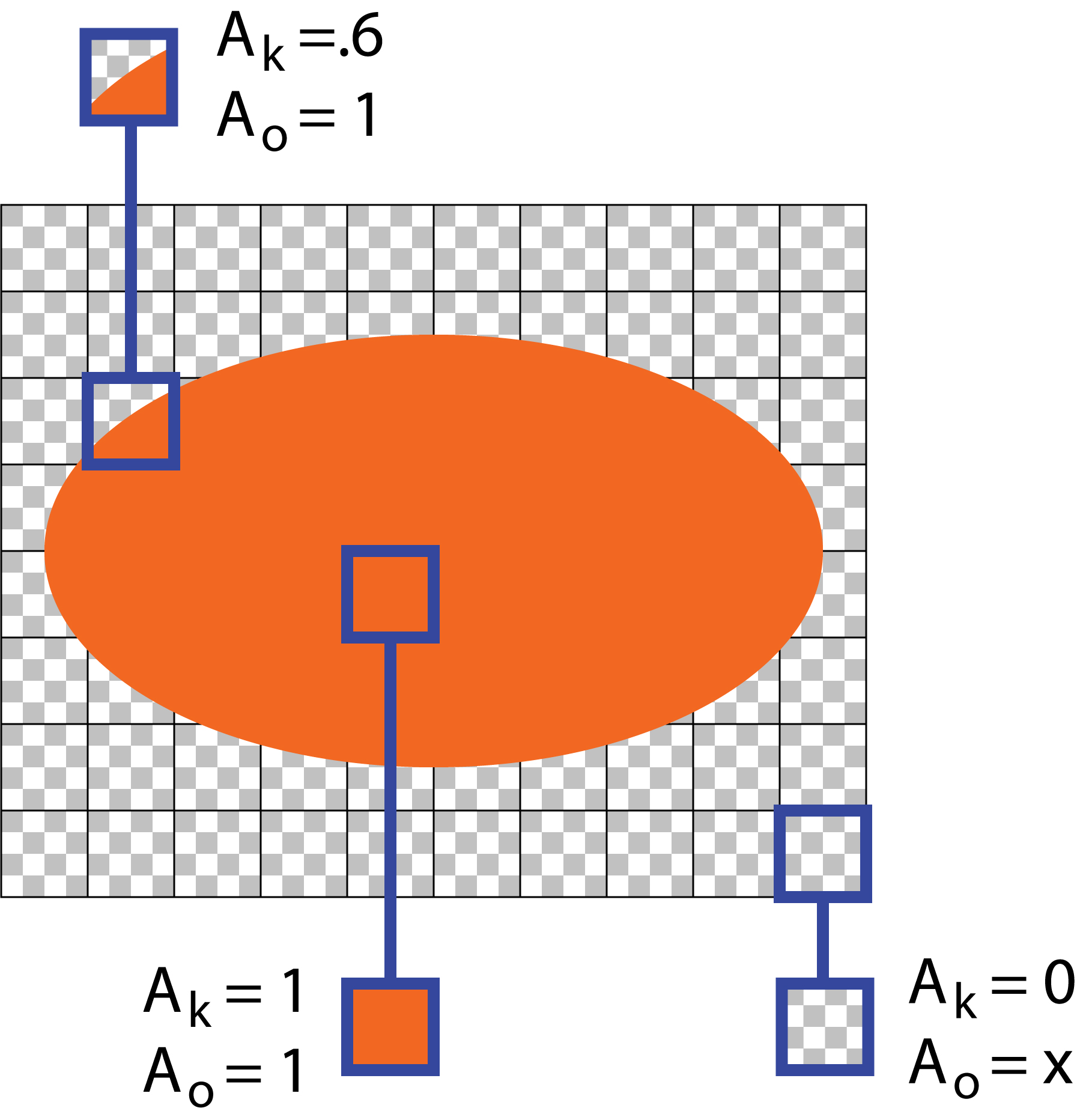
In each pixel, the coverage $A_k$ is the same. But the opacities of two of the pixels are different. In the upper-left, the opacity of the fragment is the opacity of ellipse, or $A_o=1$. The same applies to the pixel in the center that is fully covered. As before, the opacity of the completely untouched pixel in the lower right doesn't have a meaningful value, because there's no fragment there to supply an opacity.

While we're looking at these figures and talking about pixels, let's briefly return to alpha for just a moment. Note that any modern renderer will compute a value of alpha, appropriate for compositing, by multipying $A_k$ and $A_o$ together. For example, if a pixel is one-third-covered by an opaque fragment, then $\alpha = (1/3)\times 1$. Similiarly, if a pixel is completely covered by a one-third opaque fragment, the result is the same: $\alpha = 1 \times 1/3$. And if a pixel is one-fifth covered by a fragment that is one-third opaque, then 20% of the pixel is blocking 30% of the color from beneath it, so $\alpha = .2 * .3 = .06$. This product of coverage and opacity will play an important role in the following discussion.

Composition

Let's now compose two objects, $A$ and $B$, that have each been drawn in independent layers that each started out fully transparent (that is, filled with "transparent black"). Each pixel in the layer for object $A$ has three pieces of information: the color $A_c$ (or the pre-multiplied color $a_c$), the opacity $A_o$, and the coverage $A_k$. Of course, the layers for $B$ hold the same data for that image. Here again, a color value like $A_c$ or $a_c$ refers simultaneously to red, green, and blue, or, if you prefer, a single grayscale value.

Before we begin composing pixels, we need to decide how to combine them. The classic approach of [PorterDuff84] is to presume, in the absence of additional information, that the pixels are uncorrelated in every way. Both because we can see no better suggestion, and because this assumption has been proven in the real world beyond any question, we make the same assumption here.

Notice that only the coverage information is affected by this assumption. Opacity is not, because it is connected to the color of the fragment (or fragments) inside the pixel.

Using the common "little square" model of a pixel that is 1 unit on a side, Figure 3 shows a composition stack for $A$ over $B$. In this example, we are explicitly modeling area and geometry. Again, don't think of anything here as "alpha"; we'll get back to that idea later.

Using our assumption that fragments are uncorrelated, we follow [PorterDuff84] and draw the fragments so that the upper fragment $A$ overlaps both $A_k$ percent of the area of the pixel (with an area of 1) and $A_k$ percent of the area of $B_k$ under it. This is the key thing about being uncorrelated: the fragment $A$ is assumed to have no special relationship to fragment $B$. If $A$ covers $A_k$ of the pixel's area, then it also covers $A_k$ of fragment $B$'s area.

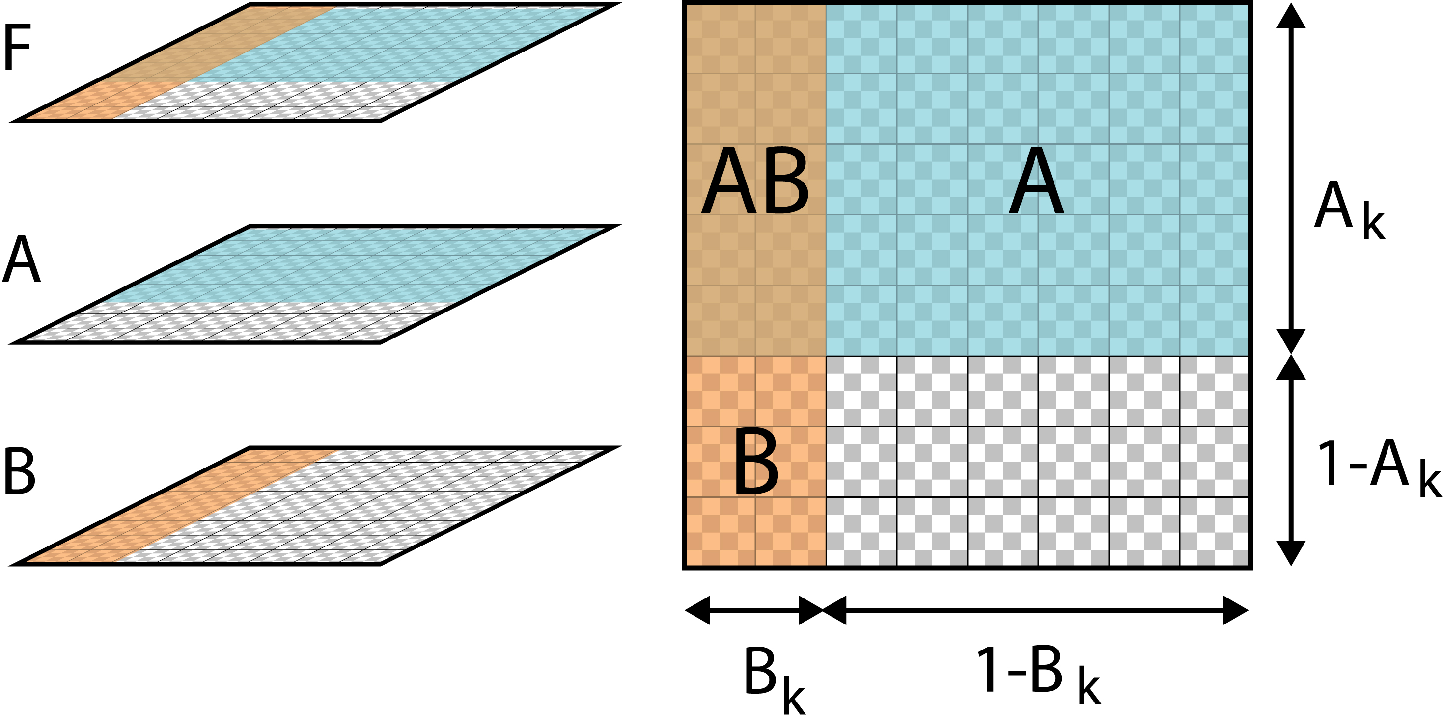
What is the final color of this pixel? Let's write the result as $F$. There are four regions to consider:

• $F_A$: The region where only $A$ is present.
• $F_B$: The region where only $B$ is present.
• $F_{AB}$: The region where both $A$ and $B$ are present.
• $F_0$: The region where neither object is present.

Let's take these in turn.

$F_A$: This rectangle has area $A_k(1-B_k)$. The color inside is $A_c A_o$. Thus the total contribution to the final pixel color is $ (F_A)_c = A_k (1-B_k) A_c A_o $

$F_B$: This area is just like the above, with $A$ and $B$ reversed. The area is $B_k(1-A_k)$, and the color is $B_c B_o$. Thus the total contribution to the final pixel color is $ (F_B)_c = B_k (1-A_k) B_c B_o $

$F_{AB}$: This region has area $A_k B_k$. The color contributed by $A$ is $A_c Ao$ and that from $B$ is $B_c Bo$. All of $A$'s color is preserved in $F$, but because $A$ has an opacity of $A_o$, it only allows $(1-A_o)$ of the color from $B$ to pass through it. So the total contribution to the final pixel color is $(F_{AB})_c = A_k B_k (A_c A_o + (1-A_o)B_c B_o)$.

$F_0$: Of course, because neither fragment contributes to $F_0$, the contribution to the final pixel from this area is 0.

The New Pixel's Color

To find the new pixel color, we merely add these four terms together:

$$ \begin{align} F_c &= (F_A)_c + (F_B)_c + (F_{AB})_c + (F_0)_c \\ &= A_k (1-B_k) A_c A_o + B_k (1-A_k) B_c B_o + A_k B_k (A_c A_o + (1-A_o)B_c B_o) + 0 \\ &= A_c A_k A_o + (1 - A_k A_o) B_c B_k B_o \end{align} $$

This looks very familiar. We can make it even more familiar by implying multiplication of terms by multiplication of subscripts, e.g., $A_{ko} = A_k A_o$. Then we can write this as

$$ F_c = A_{ko} A_c + (1 - A_{ko}) B_{ko} B_c \;\;\;\;\;\;\;\;\;({\rm Eq.\;}5) $$ If we assume for the moment that $A_\alpha = A_{k o}$ and $B_\alpha = B_{k o}$, then this looks like the standard version of over for pre-multiplied pixels $a$ and $b$, producing a pre-multiplied result $f$: $$ f = a + (1-A_\alpha) b $$

But before we make that leap, let's look at what happens when we want to compose $F$ over another image $G$ (what Smith calls the second-composition problem). To perform that operation, we need to know how much of $F$ to add to $G$ (in terms of the last equation, that would be $F_\alpha$).

Finding $F_k$ and $F_o$

Coverage

The geometry term is easy: it's merely the total amount of the pixel covered by $A$ and $B$. We can read that right off of Figure 3. In this calculation, it doesn't matter if $A$ is over $B$ or vice-versa:

$$ \begin{align} F_k &= A_k + (1-A_k)B_k \\ &= B_k + (1-B_k)A_k \\ &= A_k + B_k - A_k B_k \;\;\;\;\;\;\;\;\;({\rm Eq.\;}6) \end{align} $$

Opacity

Now let's look at opacity and find $F_o$. We can follow the same steps as before, again by referencing Figure 3. The amount of opacity added in by the region $A$ is given by the area of that region, $A_k(1-B_k)$ times the opacity in that region, $A_o$. Regions $B$ and $0$ follow the same pattern:

$$ \begin{align} (F_A)_o &= A_k (1-B_k) A_o \\ (F_B)_o &= B_k (1-A_k) B_o \\ (F_0)_o &= 0 \end{align} $$

I left $(F_{AB})_o$ off the list, because I don't want to take anything for granted. Let's analyze the opacity of region $AB$ by thinking about it in terms of transparency.

Consider two transparent sheets of plastic, $A$ and $B$. Suppose $A_o = .3$, meaning it lets through 70% of the color trying to pass through it, and $B_o = .4$, so it lets through 60% of the color. We'll stack $A$ over $B$ and look at a swatch of color with value 1 placed beneath them, as in Figure 4.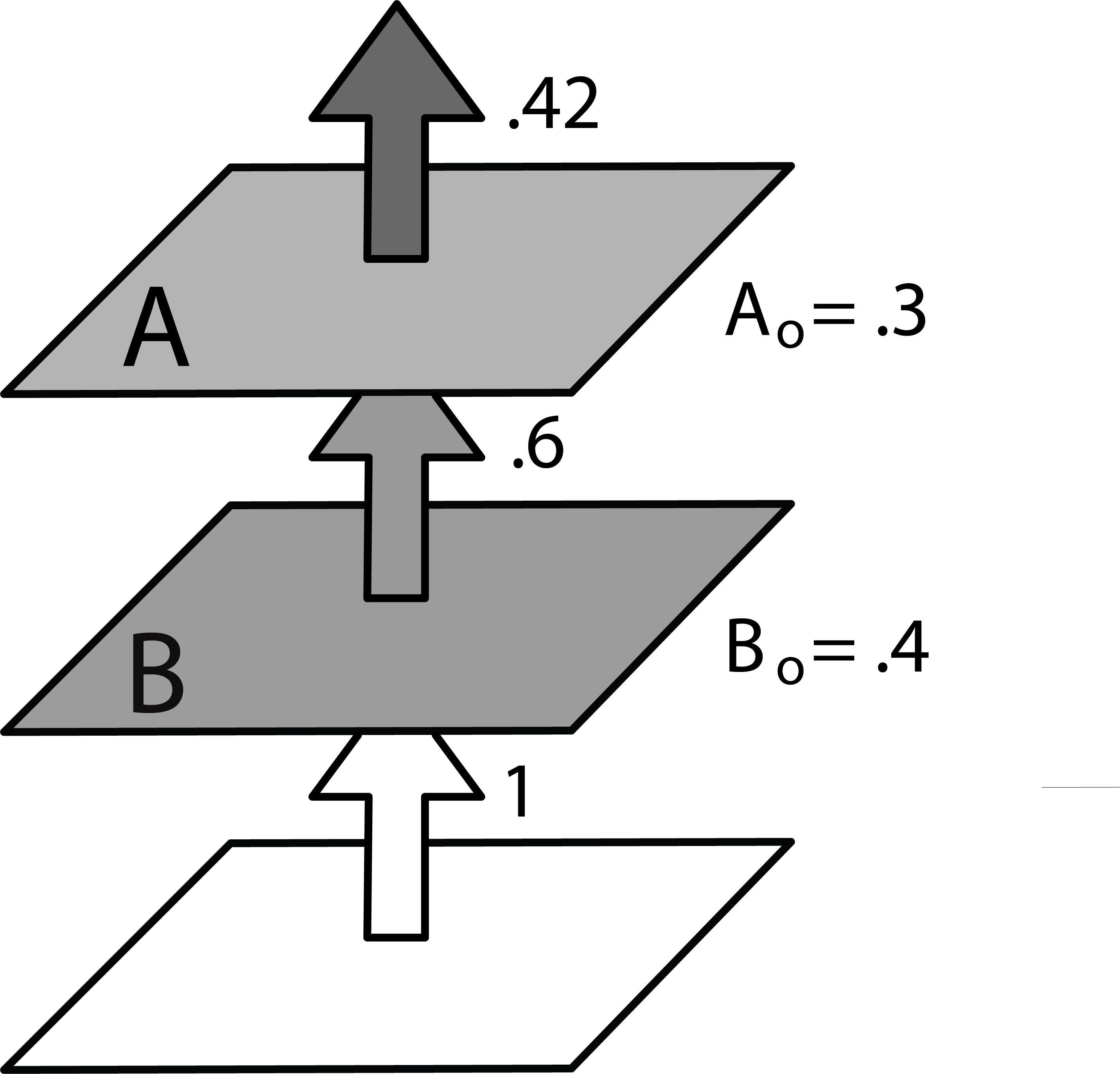

Layer $B$ has an opacity $B_o$, so it passes through $1-B_o$ of the color beneath it. The same is true of $A$. For convenience, let's write these as transparency values with the subscript $t$, so that $A_t = 1-A_o$ and $B_t = 1-B_o$. Thus the combined transparency is the product of the two components, $A_t B_t$.

In other words, transparencies are commutative: looking at the world through a 20% filter in front of a 35% filter gives the same results as the other way around.

So the opacity in region $AB$ is merely 1 minus the opacity, or $1-(A_t B_t) = 1-((1-A_o)(1-B_o))$. We can rearrange this to find:

$$ 1-((1-A_o)(1-B_o)) = A_o + (1-A_o)B_o $$

Multiplying this by the area of region $AB$ we get the opacity contributed by that region:

$$ (F_{AB})_o = A_k B_k (A_o + (1-A_o)B_o) $$

Putting the four pieces together, we have

$$ \begin{align} F_o &= (F_A)_o + (F_B)_o + (F_{AB})_o + (F_0)_o \\ &= A_k (1-B_k) A_o + B_k (1-A_k) B_o + A_k B_k (A_o + (1-A_o)B_o) \\ &= A_k A_o + B_k B_o - A_k B_k A_o B_o \end{align} $$

This last expression has a very nice geometric interpretation. It tell us that that to find the total opacity, add the opacity contributed by $A$, given by $A_k A_o$, to the total opacity contributed by $B$, given by $B_k B_o$, but then notice that we've added the region $AB$ twice, so subtract that region once by removing $A_k B_k A_o B_o$.

It's tempting to stop here, but notice that our final expression above is being weighted by area-based factors, and we're not normalizing afterwards. In other words, we're mixing the opacities together as specified by the areas, and those areas are getting included in the final value. As we saw earlier in the Blending section, to remove the influence of the area terms in the result, we need to divide by their sum:

$$ F_o = \frac{A_k A_o + B_k B_o - A_k B_k A_o B_o }{A_k + B_k - A_k B_k} $$

We've seen that denominator before. Of course, it's just the total area of the fragments, which we found in the last section as $F_k$. So the normalized value for the opacity is then

$$ F_o = \frac{A_k A_o + B_k B_o - A_k B_k A_o B_o }{F_k} \;\;\;\;\;\;\;\;\;({\rm Eq.\;}7) $$

Combining Opacity and Coverage

When we compose $F$ over some other image, at each pixel $F$ has coverage $F_k$ and opacity $F_o$. For the same reasons that the original rendering produced a value of alpha at pixel equal to the coverage of that pixel times the fragment's opacity, the value of alpha that we need to apply to $F$ in order to use Equations 2, 3, or 4 is $F_{ko}$. In other words, to compose $F$ over some other image $G$ using Equations 2 through 4, image $F$ takes the place of $A$, so we use $F_{ko}$ as the value of $A_\alpha$.

To find $F_{ko}$ we just multiply $F_k$ and $F_o$. Those terms are given by Equations 6 and 7, so let's gather them together here:

$$ \begin{align} F_o &= \frac{A_k A_o + B_k B_o - A_k B_k A_o B_o}{F_k} \\ F_k &= A_k + B_k - A_k B_k \end{align} $$

Notice that both of these expressions are symmetric in $A$ and $B$. So the order of composition matters when we compute colors, but the resulting opacity and coverage are identical for $A$ over $B$ and $B$ over $A$.

Let's now find the product $F_{ko}$:

$$ \begin{align} F_{ko} &= F_k \frac{A_k A_o + B_k B_o - A_k B_k A_o B_o}{F_k} \\ &= A_{ko} + B_{ko} - A_{ko}B_{ko} \\ &= A_{ko} + (1 - A_{ko}) B_{ko} \;\;\;\;\;\;\;\;\;({\rm Eq.\;}8) \end{align} $$

This looks very familiar. Compare Equations 3 and 8:

$$ \begin{align} F_\alpha &= A_\alpha + (1-A_\alpha) B_\alpha \\ F_{ko} &= A_{ko} + (1 - A_{ko}) B_{ko} \end{align} $$

We've already seen that $F_{ko}$ is the value we use for $A_\alpha$ in Equation 3 when compositing $F$ over another image.

In other words, we've reached our goal: $F_\alpha = F_{ko}$.

Discussion

We have found that when creating $F = A {\rm \;over\;} B$, we can track each pixel's coverage $F_k$ and opacity $F_o$ independently. We also found that the value of $F_\alpha$ given in Equation 3 is given by the product of the coverage and opacity, $F_{ko}$.

The value of the process is not just that we've found another derivation of $F_\alpha$. The real payoff is that we've found what alpha represents without ambiguity.

Recall that we earlier noted that when rendering, the alpha at each pixel is the product of opacity and coverage. And we've now seen that this is always true. Even when we've composed images together to create a composite, the alpha at each pixel in that composite is the product of that pixels's final coverage and opacity.

So the quotes at the start are all correct, but they're only a few of ways we can think of alpha. Suppose you have a pixel with an alpha value of $\alpha=0.24$. You know that this is the product of the total coverage and total opacity, but you don't know how either of these values are distributed over the pixel. A few pairs of values that multiply to $0.24$ are shown in Figure 5, along with a few of the infinite pixels they could be describing.

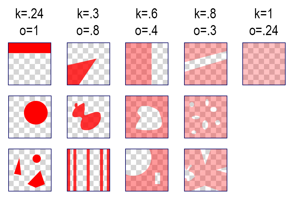
So if we have an alpha of, say, $0.24$, we can indeed think of it as a single opaque shape that occupies about a quarter of the pixel's area, as in the top left of Figure 5. Or we can interpret it as an opacity value for a fully-covered pixel, as in the the upper-right of Figure 5. This is why pictures like Figure 3 are valid: they're just one of the many ways to draw a pixel with a given value of $\alpha$.

But we can interpret $\alpha$ in any of an infinite number of other ways. Essentially we can treat the pixel as any collection of shapes, each of which have any opacity, as long as the product of the total opacity and total coverage is equal to alpha.

Thus we're free to adopt the viewpoint in [Smith84], that when rendering all geometry is lost and only opacity remains (right column of Figure 5). But we're just as free to think that all opacity is lost and only area remains (left column of Figure 5). Or we can choose anything else in between.

Figure 6 shows just a few more possible pixels that have the same alpha as in Figure 5. As far as alpha is concerned, every one of the pixels in Figures 5 and 6 are equally likely to represent the "true" appearance of the pixel (one that might be produced, say, by very high supersampling, or a very accurate fragment-based renderer). Of course, we may have additional knowledge about our images that could lead us to prefer some possibilities over others, but that uses more information than is encoded simply in a color and an alpha value.

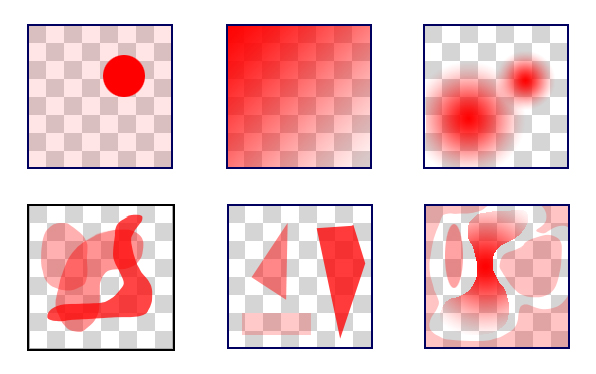
So the coverage and opacity distribution over a pixel can both be anything from a single opaque shape to a partly-transparent fractal dust, among infinite other possibilities. As long as the total coverage and opacity multiply to a pixel's alpha, we're free to distribute that opacity and coverage in any way we want.

Suppose you don't know anything about how a pixel was generated, but you wanted to choose a model of the pixel for use in other calculations. Personally, if I gather together parsimony, uniformity, isotropy, simplicity, and Occam's Razor, put them in a bag along with Figures 5 and 6, and shake, the upper-right of Figure 5 is what falls out for my model of alpha: the whole pixel is covered (so $A_k=1$) with a layer of opacity $A_o = \alpha$. This seems to make the fewest possible assumptions about the distribution of both coverage and opacity.

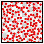
First runner-up would be something from the left column of Figure 5. Those patterns come in second because everything there requires inventing some kind of shape (or shapes) to represent the pixel's coverage. With nothing else to go on, I wouldn't know what shape (or shapes) would be best. I think I'd prefer a Poisson distribution of small circles (or even Gaussian blobs), so I'd at least get close to something that didn't favor any specific orientation or structure. Figure 7 illustrates the idea. Here the opacity is 1 (so $A_o=1$) and the sum of the areas is the coverage is $A_k = \alpha$. But if I knew something about the geometric structure of the source material that generated the pixel, I'd definitely try to use that information to design pixel geometry that more closely matches that of the input.

Conclusion

We have shown that the popular idea that alpha represents either coverage or opacity, depending on convenience, is correct, but incomplete. A pixel's alpha actually represents the product of the total coverage and the total opacity. We are free to distribute those qualities throughout the pixel in any way we want.

References

[Blinn94] Blinn, James F, "Compositig, Part 1: Theory", IEEE Computer Graphics and Applications, September 1994

[PorterDuff84] Porter, Thomas, and Duff, Tom, "Compositing Digital Images", Computer Graphics (Proc. SIGGRAPH 84), Vol 18, No 3, Jul 1984, pp. 253-259

[Smith95] Smith, Alvy Ray, "Image Compositing Fundamentals", Microsoft Technical Memo 4, August 15, 1995 http://www.cs.princeton.edu/courses/archive/fall00/cs426/papers/smith95a.pdf