Abstract

Geometric primtives are a staple of many rendering systems. They provide modelers with shapes that are easy to understand and create, yet can be easily combined and modified into more complex structures. Here we introduce a new geometric primitive called a $\textit{glob}$. It is a smooth curved shape that blends two disjoint circles or spheres of any radii. Globs are controlled with a few parameters which have immediate geometric interpretations. Globs are useful in both 2D and 3D modeling.

There's an interactive demo at the end of this document. You can jump to the demo any time! Go ahead - you can always come back and read all this stuff later!

Expanded Published Version Available

I've published a significantly improved version of this note as a paper in the Journal of Computer Graphics Techniques. I strongly suggest you read that version! I'm leaving this one available for historical reasons, and because it has the cool demo at the end.

Introduction

Almost every modeling system offers a mix of free-form and predefined shapes that can be used as starting points for more complicated models. These shapes can be broken down into three categories: primitive shapes (e.g., spheres and polygons), compound shapes (e.g., cylinders with spheres on the ends, or boxes made of multiple polygons), and procedural shapes (e.g., swept surfaces and surfaces of revolution).

Part of the design of a modeling system is choosing the right collection of these primitives. A list that's too small can be constraining, while a list that's too big can be unwieldy and bewildering.

One popular class of primitive shape combines spheres with connectors between them. These types of shapes are perfect for ball-and-stick molecules, but they are also great for nets, flexible sheets, deformable height fields, and many other applications.

The $\textit{cone-sphere}$ introduced by Max smoothly joins two non-overapping spheres with with a circular cone [Max90]. An implicit surface technique popularized by Blinn replaces each sphere with a spherically symmetric Gaussian density field called a $\textit{blob}$ [Blinn82]. The shape this produces is defined by an isosurface of this 3D field.

Both of these primitives have a lot going for them: Given two spheres, the cone-spheres require no parameters or controls, and blobs produce lovely stretching and clumping effects as the blob centers move with respect to one another.

These primitives each have drawbacks, though. Because cone-spheres have no shape parameters, they offer no variation or control, and the silhouette is always a straight line joining two circles. Blobs have more parameters, but these offer little control over the fundamental nature of the shapes they produce. For example, as two blobs pull apart the neck between them gets thinner and thinner until the two shapes disconnect, but one cannot control the length or shape of this neck. To compensate, some modeling systems allow the designer to use other shapes to generate density fields [Wyvill99]. This approach is very flexible and offers an exciting breadth of control, but that very flexibility introduces a signficant increase in complexity and effort from the designer.

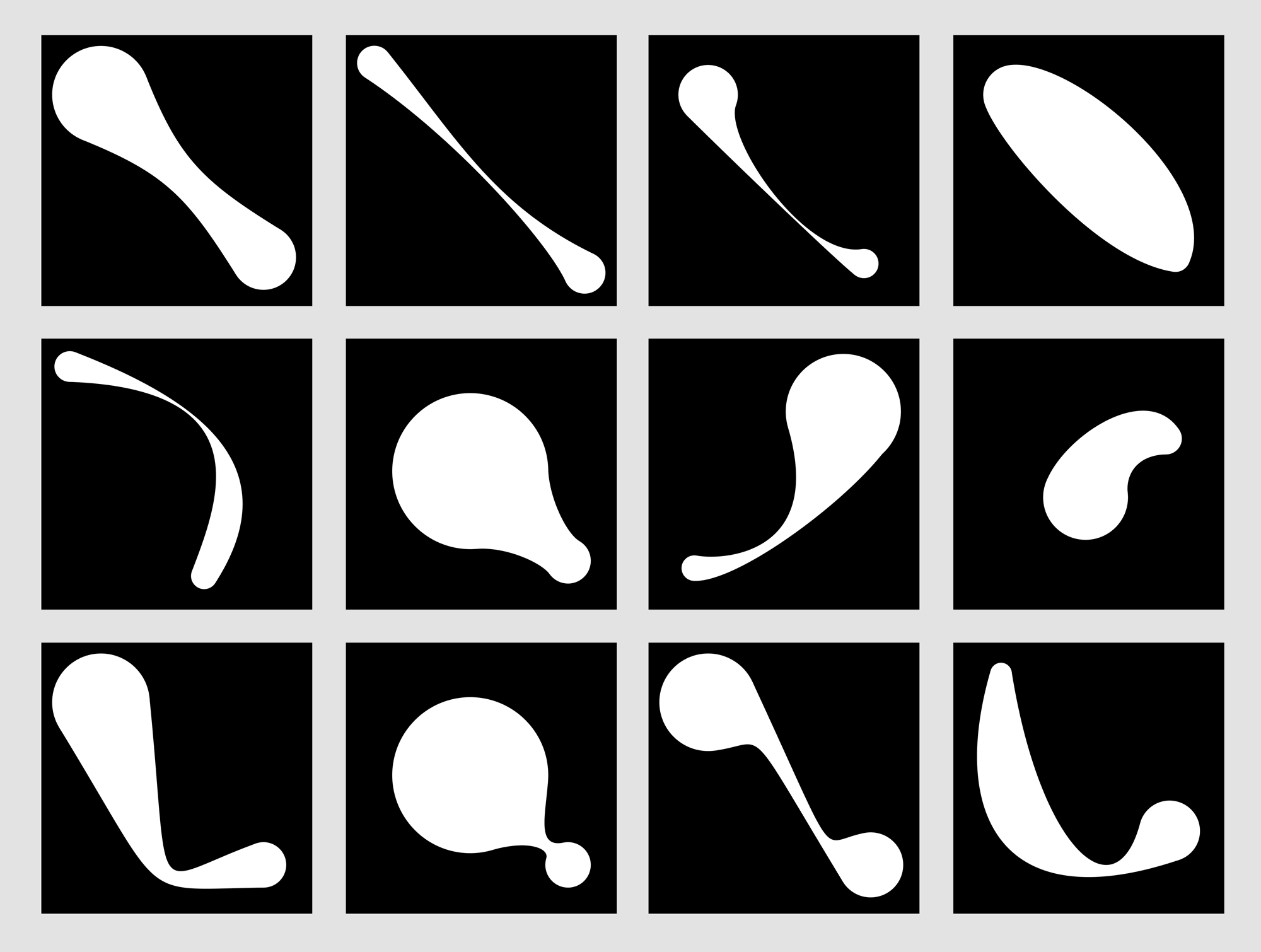
We have designed a shape that combines some of the best features of cone-spheres and blobby spheres, offering a wide range of shapes from a relatively small set of parameters. Some examples are shown in Figure 1. We produce an explicit curved neck between any two non-overlapping spheres. The neck can bulge inward or outward, and move flexibly in the space between the spheres. We can recreate classic cone-sphere and blobby effects, but we can also easily create new kinds of shapes that would otherwise be difficult to produce, such as necks that start abruptly at one end but grow gracefully at the other, and asymmetric, bulging necks.

The Geometry

The heart of the idea in 3D is that we build a Bezier surface between the two spheres. We construct the surface so that it has at least first-derivative continuity with both spheres. The designer can adjust many visual aspects of this connective surface.

The easiest way to describe the process is to represent the spheres as 2D circles in a plane, and construct a cubic Bezier curve that joins them. We can use this construction directly in 2D, to produce shapes such as those in Figure 1, or rotate the curve around the line between the circle centers to produce a 3D surface of revolution. We can include the circles at both ends in this surface of revolution, of course, creating a single explicit 3D shape.

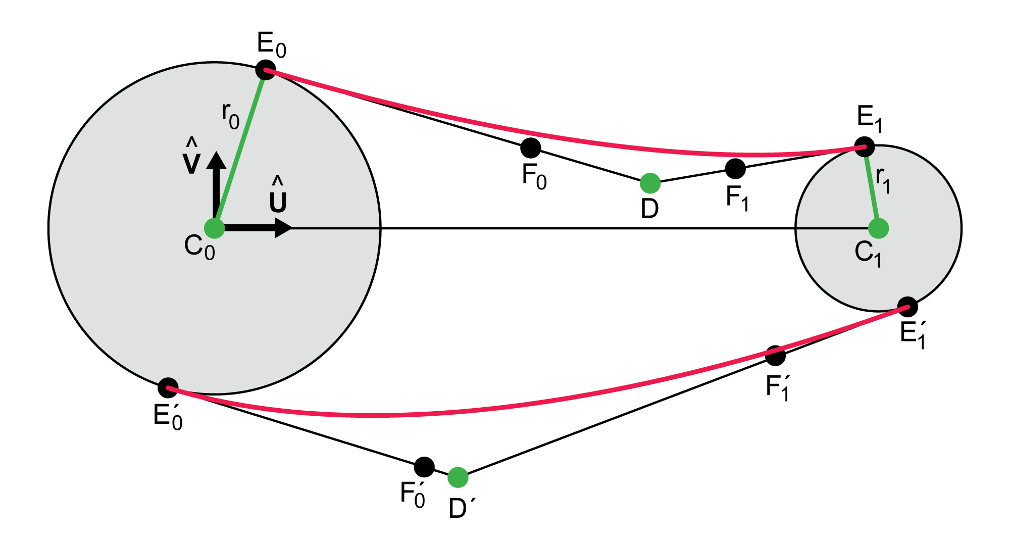
Figure 2 shows the basic idea. We call the two circles $C0$ and $C1$, with respective centers $C_0$ and $C_1$ and radii $r_0$ and $r_1$. It is tempting to simplify the geometry by placing $C_0$ at the origin and $C_1$ at point $(1,0)$, and indeed one can do this with no loss of generality. As a practical matter, though, we have found that it's more convenient to solve the general case using coordinate-free vector techniques. This lets us produce results that are immediately applicable in both 2D and 3D, without the need to write additional code for scaling, rotation, and translation after the construction is done.

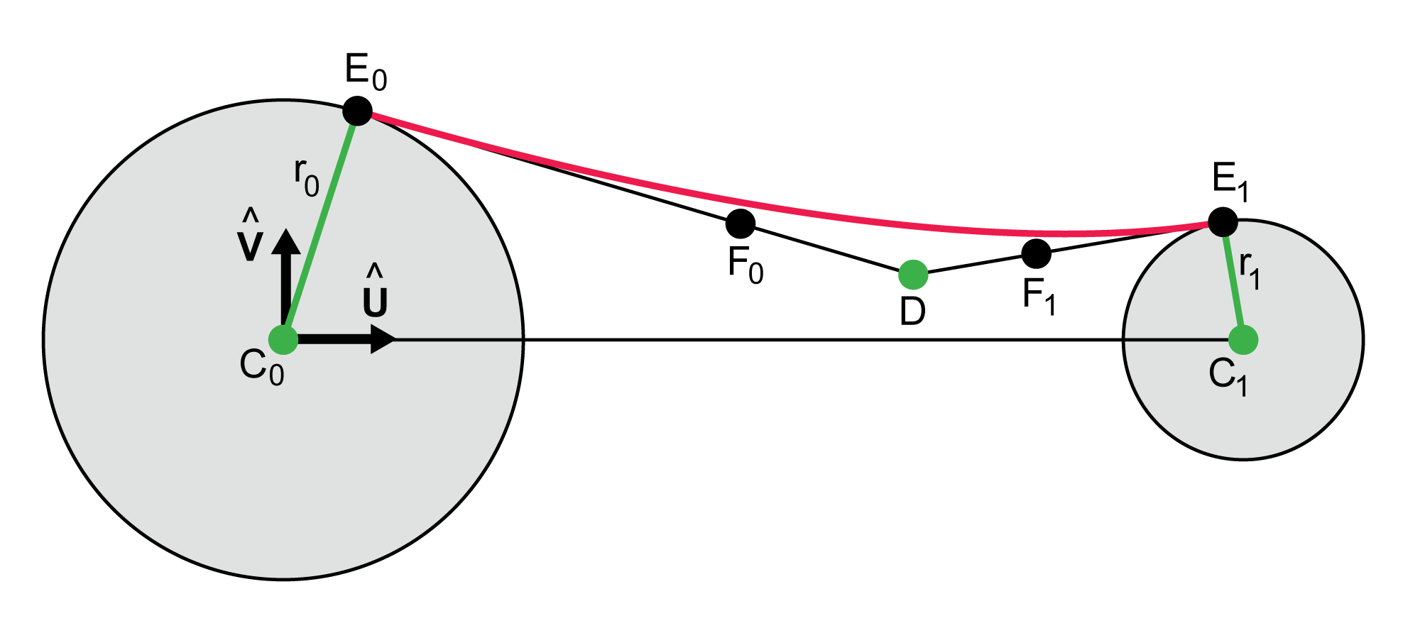
The first step is to introduce a local coordinate system. We create the normalized vector $\hat{\mathbf{U}}$ on the axis from $C_0$ to $C_1$:

The narrowest (or widest) part of the neck is given by the the point $D$, which the designer can place anywhere outside of the spheres. To create our Bezier curve, we draw lines from $D$ to each circle so that they are tangent to the circle. In the figure, these points are labeled $E_0$ and $E_1$. They serve as the endpoints for the Bezier curve.

To build a cubic Bezier curve we need two control points. We locate these on the lines $(E_0,D)$ and $(E_1,D)$, and are marked $F_0$ and $F_1$ in the figure. The locations of $F_0$ and $F_1$ are found using two designer-specified scalars that tell us where they should be placed along their respective lines.

The curve we want is then given by $(E_0, F_0, F_1, E_1)$. By construction, this has first-derivative continuity with the circles at both ends.

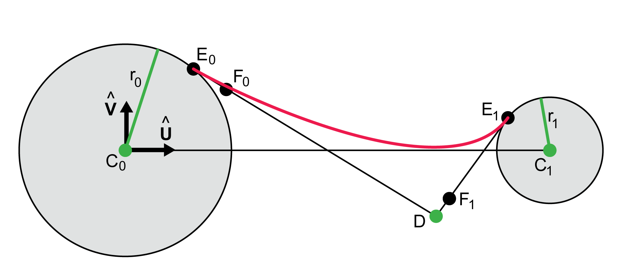
Note that $D$ can be literally anywhere that is not within either of the two circles. It can be below the line $(C_0,C_1)$ or far outside the convex hull of the circles.

It is fun (and instructive) to work this out as a problem in plane geometry, creating a web of right triangles and using trig to find points $E_0$ and $E_1$. However, a vector approach is much simpler and robust. Figure 3 shows the geometry. We can think of Figure 3 as a subroutine: given a circle with center $A$ and radius $r$, and a second point $B$ that is outside the circle, find a point $P$ on the circle such that the line $(P,B)$ is tangent to the circle. As the figure shows, there are two points that fulfill that condition, so we choose a point using one more argument to our routine (discussed in a moment).

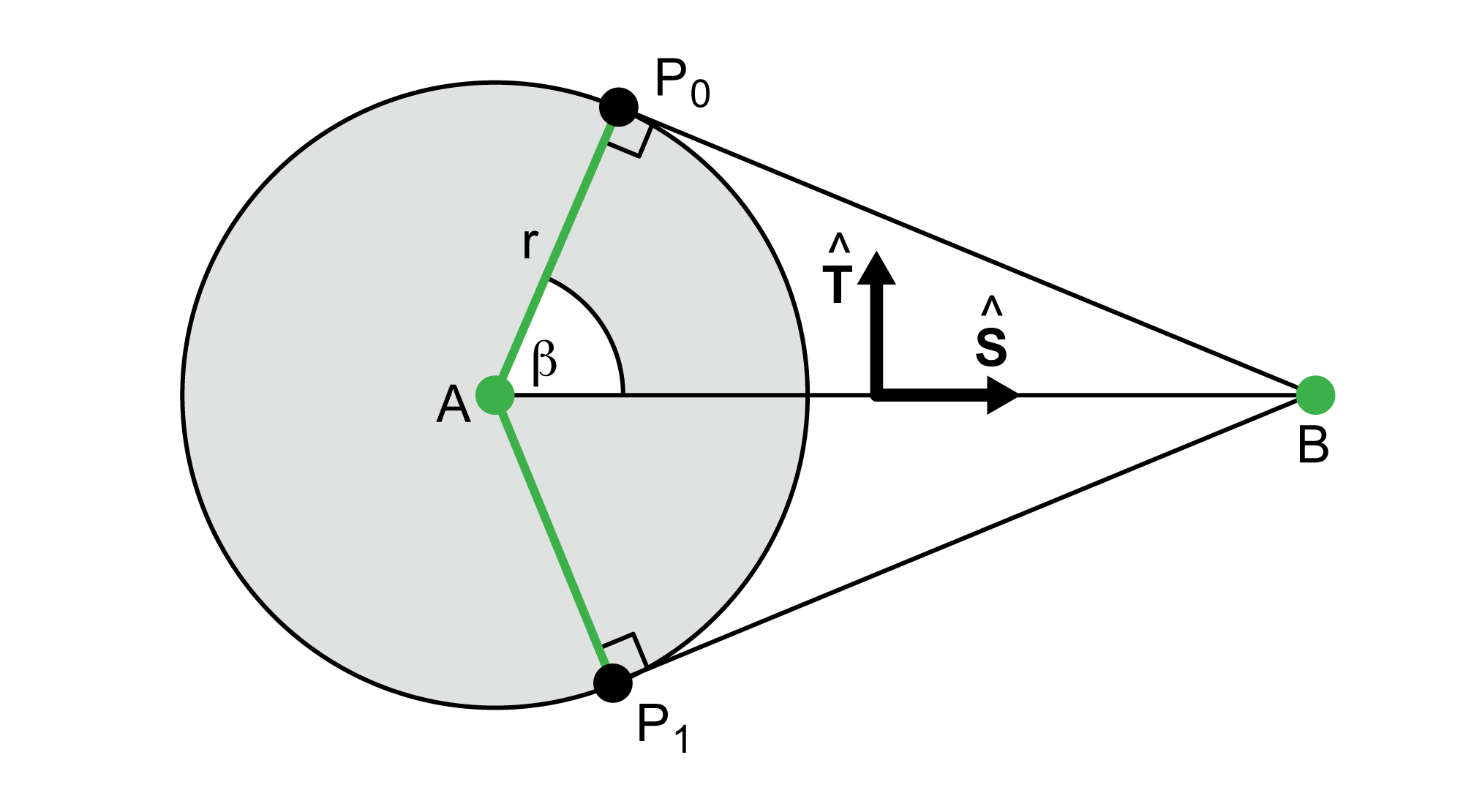
We begin by constructing a frame of perpendicular unit vectors $\hat{\mathbf{S}}$ and $\hat{\mathbf{T}}$, where $\hat{\mathbf{S}}$ points from $A$ to $B$. To find $P_0$, we only need to find angle $\beta$. We know one leg and the hypotenuse of right triangle $A P_0 B$. The length of the remaining leg is provided by Pythagoras:

Now we can find $\beta$ using arc-tangent: $$ \beta = \tan^{-1}(|P_0 B|\,/\,r) $$

From this, we can create the two points $P_0$ and $P_1$, one on each side of of $\hat{\mathbf{S}}$. The expressions are identical except that we add a scaled version of $\hat{\mathbf{T}}$ when forming $P_0$ and subtract it for $P_1$:

Both of these points satisfy our initial criteria. We mentioned above that we have one additional argument that lets us pick the one we want. This argument specifies whether we want the one that is on our left or right as we stand at $A$ and look towards $B$. To find which point lies on which side, we find two cross products, and take the sign of their $z$ component:

By construction, one of these values will always be positive (on our left) and the other will always be negative (on our right). So if we want the left-hand point we return $P_0$ if $s_0 > 0$, otherwise we return $P_1$. For the right-hand point, we return $P_0$ if $s_0 < 0$, else $P_1$.

This method provides us with points $E_0$ and $E_1$, which provide the endpoints of our Bezier curve. The next step is to find the internal control points $F_0$ and $F_1$.

To find $F_0$, the designer specifies a scalar value $a_0$. This gives us a point on the line from $E_0$ (when $a_0=0$) to $D$ (when $a_0=1$). This is something of a $\textit{tightness}$ parameter, since it pulls the curve more or less forcefully towards the point $D$. We find $F_1$ in the same way, using $a_1$:

We can now draw the cubic Bezier curve $(E_0, F_0, F_1, E_1)$. This has first-derivative continuity with the circles at both ends.

For 3D work, we can rotate this curve around the line $(C_0,C_1)$ to produce a surface of revolution.

Because point $D$ can be anywhere outside of the two spheres, we can produce a wide range of squeezes and bulges. Because the tightness parameters $a_0$ and $a_1$ are independent, we can individually adjust how quickly the neck forms at each end, as shown in Figure 4.

When working in 2D it's fruitful to produce a lower Bezier curve independently of the upper one. We can identify the values for this curve with primes. Thus the user can place a point $D^\prime$ anywhere outside the two spheres, and from that we will find points $E_0^\prime$ and $E_1^\prime$. Using tension parameters $a_0^\prime$ and $a_1^\prime$, we find control points $F_0^\prime$ and $F_1^\prime$, giving us a new Bezier curve. These two curves can interact in many ways, producing a generous variety of shapes, as shown in Figure 1. Of course, all of these can still be rotated around the line $(C_0,C_1)$ to produce 3D shapes, though if the resulting surface is opaque much of the interaction between the two curves may be lost.

Discussion

User Interface

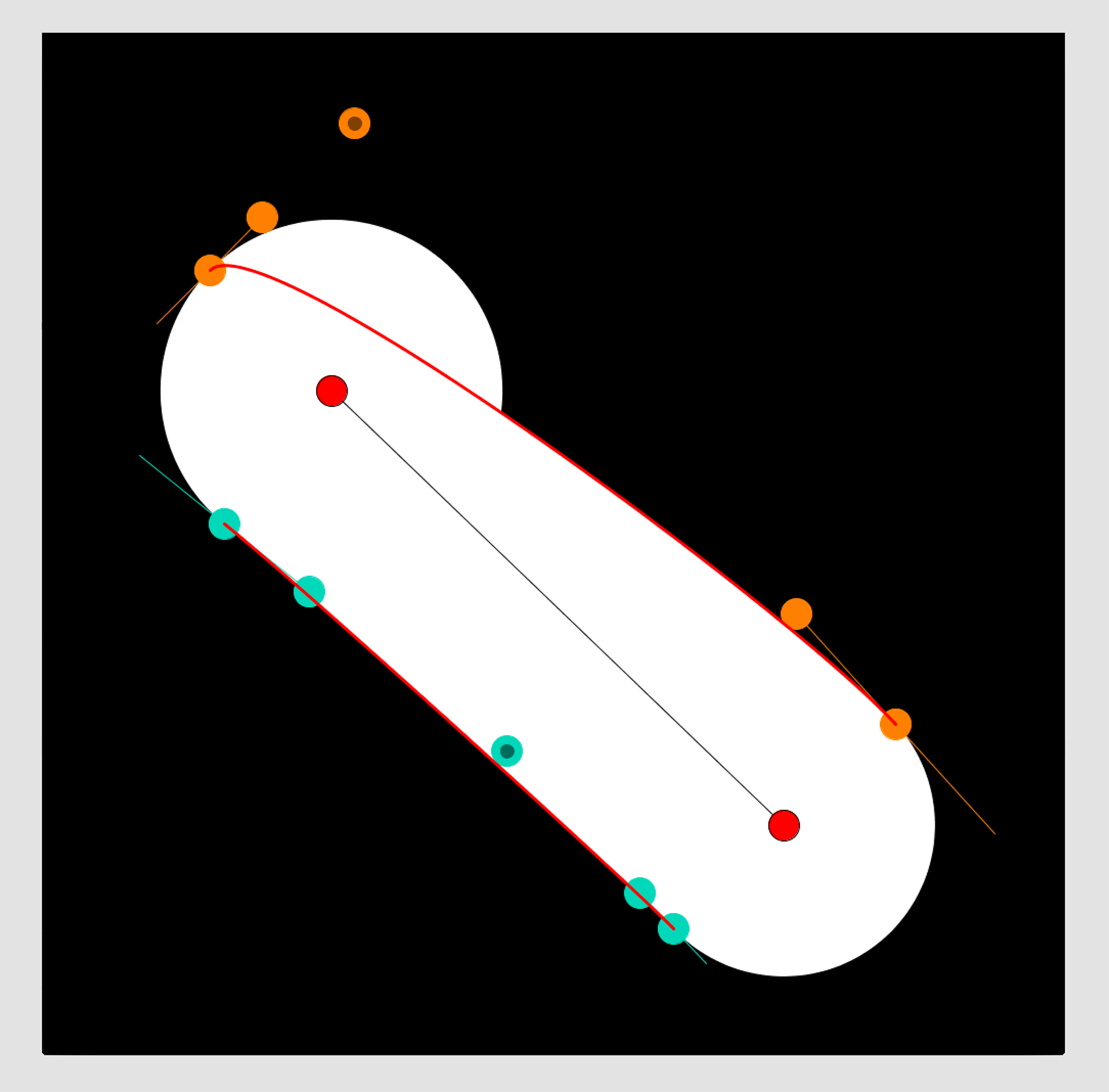
We have built a small stand-alone design program for making globs. Using this program, the designer can specify all the glob parameters interactively. As shown in Figure 6, we draw small dots at the center of each circle, and at the points $D$ and $D^\prime$. The designer can simply click and drag any of these points around to create the basic geometry. The system interactively computes the locations of the points that define the Bezier curve, and it also draws the four points of each curve.

The other points are constrained in their movements. To set the radius, the designer may move points any of the $E$ points (those on either circle's perimeter) towards or away from their corresponding circle's center. Because both pairs (such as $E_0$ and $E_0^\prime$) lie on the same circle, moving one towards or away from the circle center will cuase a corresponding motion in the other.

The designer can also grab $F_0$ and drag it anywhere on the line $(E_0, D)$, including outside the segment between the two points. Of course, the same holds for the other versions of $F$ points as well.

The system uses the locations of these points to infer the geometry of the glob. The circle centers can be used immediately. The radius of each circle is given by the distance from a circle center to either of its $E$ points (as mentioned above, moving either $E$ point causes the other to move so they are both the same distance from the circle center). The $a$ values are found from their corresponding $E$ and $F$ points. For example, $a_0 = |F_0-E_0|/|D-E_0|$, where we use signed lengths.

Pressing a key allows the designer to turn these interfaces elements on and off.

We have found that when building globs in a larger system that may include other shapes, sometimes one will want to use one or two pre-existing circles (or spheres) as endpoints for a glob. It's important to give a designer that option in such an environment.

Cusps and Loops

The tension parameters $a_0$ and $a_1$, and their primed counterparts, can be made large enough that the Bezier curve they control forms a cusp, or even a loop. It is possible to detect both of these cases [Stone89], and one could limit either the values of these parameters, or the location of point $D$, or both, to prevent cusps and loops. We prefer to leave the values unconstrained, so the designer is free to explore the shapes that result from setting the tension parameters to negative or large positive values.

Unexpected Corners

Our geometry for finding the tangent points is robust and fast, but it can produce a sharp corner where one might expect a smooth blend. This is because although the curve will be tangent to the circle at the point of type $E$, depending on the tension parameters and the location of $D$ the curve may be shaped so that it does not wrap around the circle, but instead passes through it. The result is what appears to be a corner where the neck emerges from the circle, as shown in Figure 7.

One could detect this condition (perhaps by moving very slightly along the curve and testing to see if that point is inside the circle), and then enforce constraints to avoid it. But just as with cusps and loops, we don't try to prevent the designer from creating such globs, because they can be useful.

Tangents, Normals, and Offset Curves

A nice feature of globs is that they have easy-to-compute tangent and normal vectors. For points on the circular ends, finding tangents and normals is trivial: the normal is merely the unit vector from the point on the circle to the center of the circle, and the tangent is its perpendicular. It's also easy to find these vectors along the Bezier curves. The tangent is given by the standard equation for the tangent to a Bezier curve at a given point, and the normal is its perpendicular.

We can use use these normals to approximate an offset curve. It is well known that one cannot explicitly construct a Bezier curve that is the offset of another [Pomax15], but there are many approximating alternatives. One of the simplest is to evaluate the curve at many points and find the normal at each point. An approximate offset curve can be producing simply by scaling the normals and joining them together as a spline.

The glob offset curves in Figure 8 were constructed in this way. We sampled many points, found the normals, scaled them, and connected the endpoints together in a single closed Catmull-Rom curve.

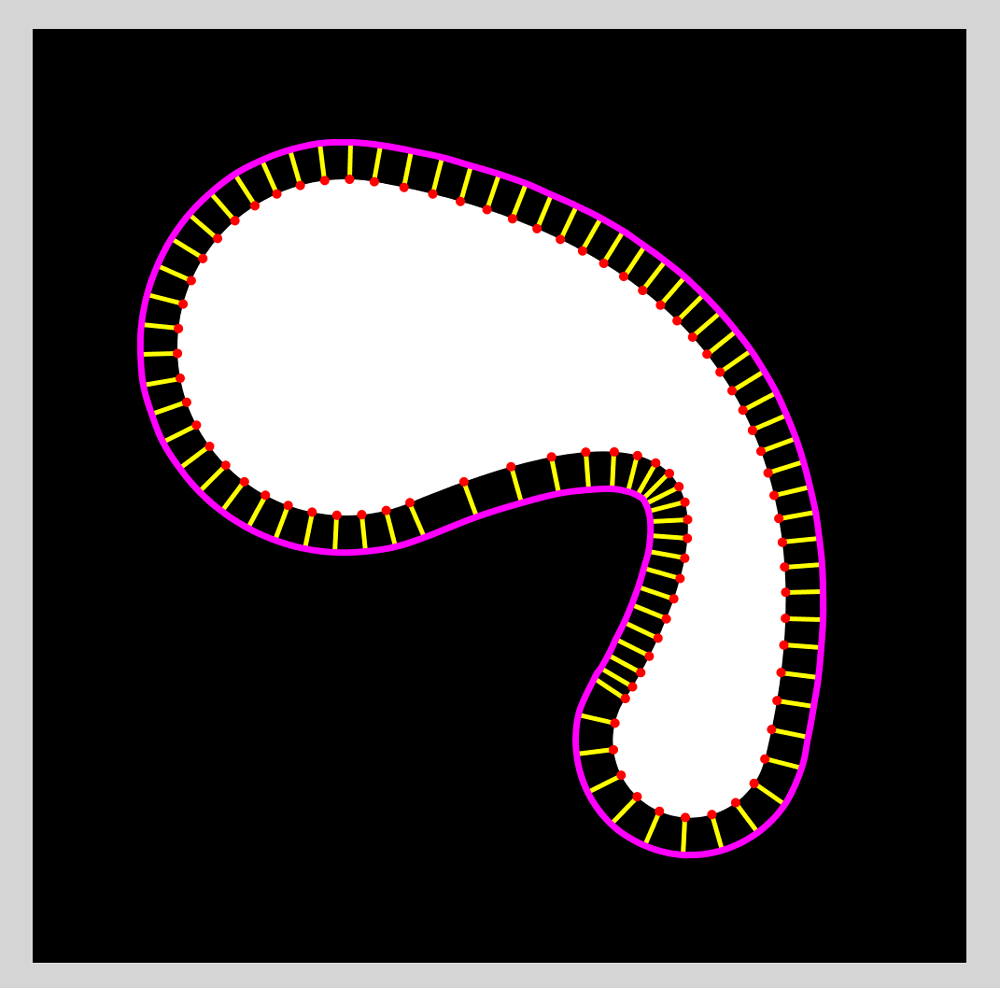
One note of caution when working with this approach, though, is that one must remember that Bezier curves are not uniformly parameterized. That is, taking equal steps of the input parameter (say $t$ going from $0$ to $1$ in steps of $.1$) will usually $\textit{not}$ result in equally-spaced points along the curve. This phenomenon is easily visible in the inner curve in Figure 9.

When the sampling density of points along the curve is low, this non-uniform spacing has the risk of creating artifacts in the resulting offset curve. Probably the easiest way to resolve the problem is to use more points. Another option is explictly adjust the evaluation parameter for the Bezier curve so that it corresponds to arclength along the curve. This can be done by pre-computing the approximate arclength at many points along the curve, and then looking up each input value in that table, producing a new evaluation parameter that produces a point that is at the desired distance along the curve. A further discussion of this technique along with an implementation may be found in [Glassner14].

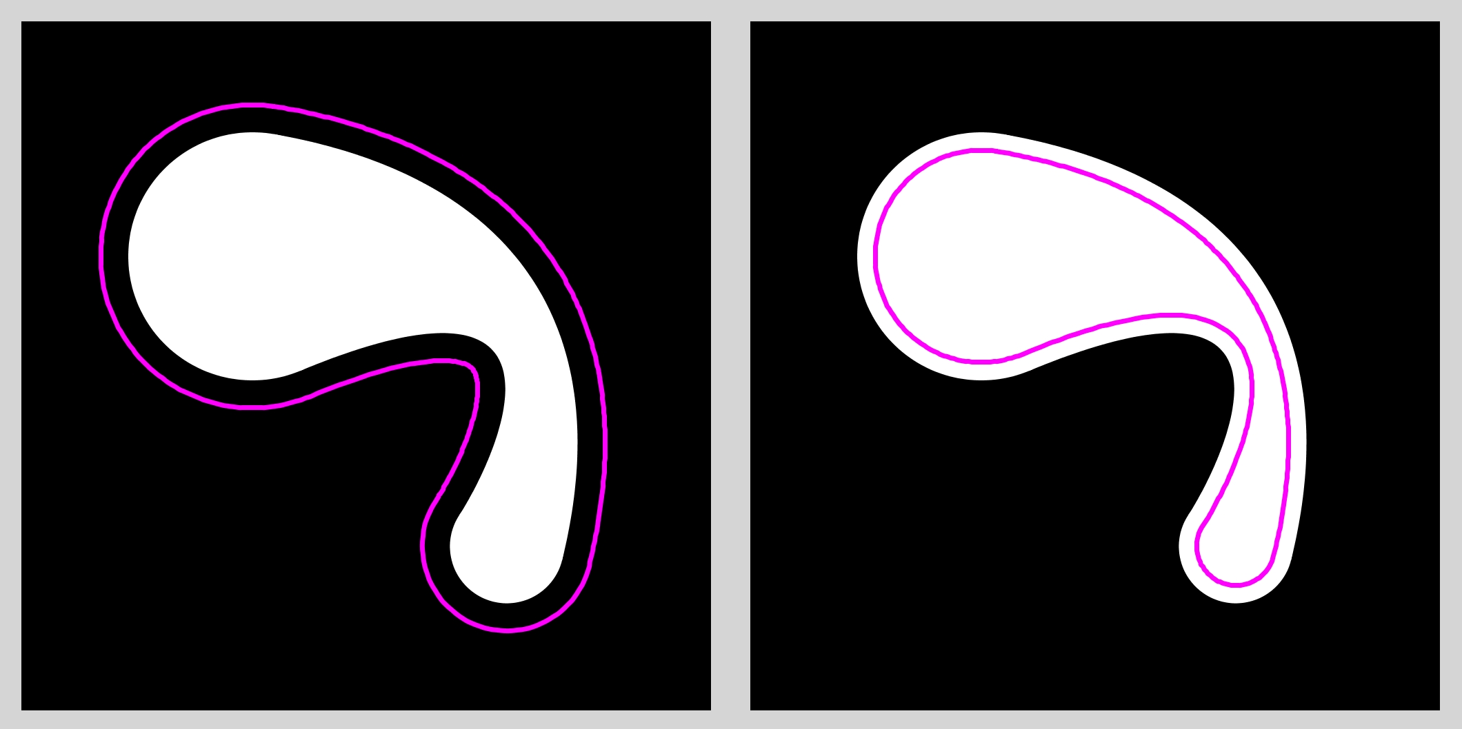
Depending on the particular curve shape and offset amount, offset Bezier curves can exhibit loops, swallowtails, and other unexpected features. In particular, tight turns and large offsets reliably lead to cusps. The upper-left of Figure 10 shows one such example. Notice that the inner offset for this same glob, shown in the upper-right, does not share the swallowtail in the outer offset. These phenomena are a natural property of offset Bezier curves, and have nothing to do with the glob's particular geometry or shape. In general, as with the cusps and loops mentioned above, it's a judgment call by the designer to determine whether to accept these features, or to eliminate them by changing the distance of the offset (lower-left of Figure 10) or changing the shape (lower-right of Figure 10).

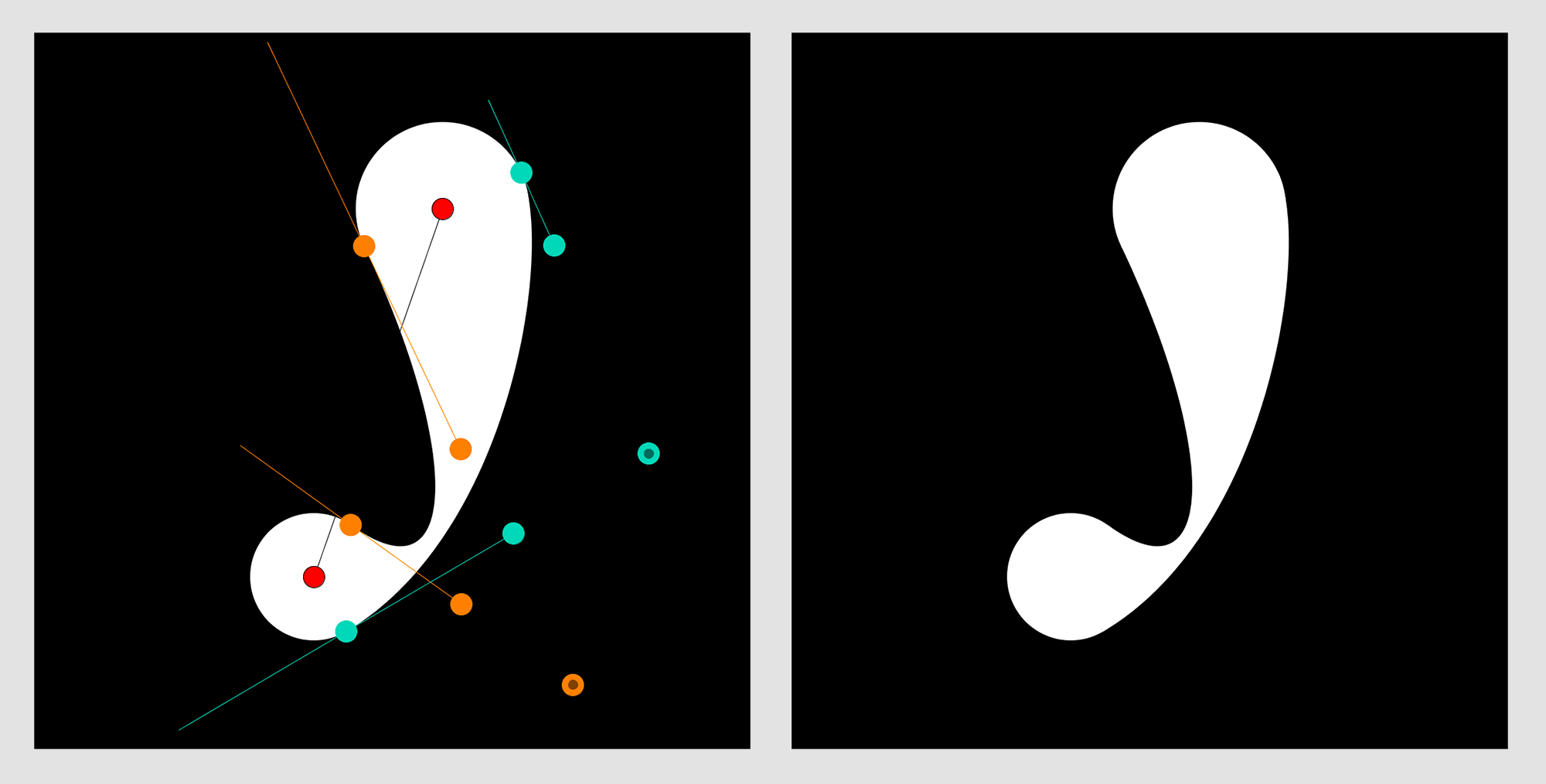
Smoothing Multiple Globs

An interesting issue arises when two globs share a common end (that is, the same circle or sphere). In some cases, they can produce a sharp corner where they overlap, as shown in the left of Figure 11. This is no different than when any two primitives overlap: there is no natural or automatic blending. And in many situations this contrast between smooth curves and sharp corners can be attractive. But because globs normally have a very smooth nature, there are times when we would like them to blend together smoothly as well.

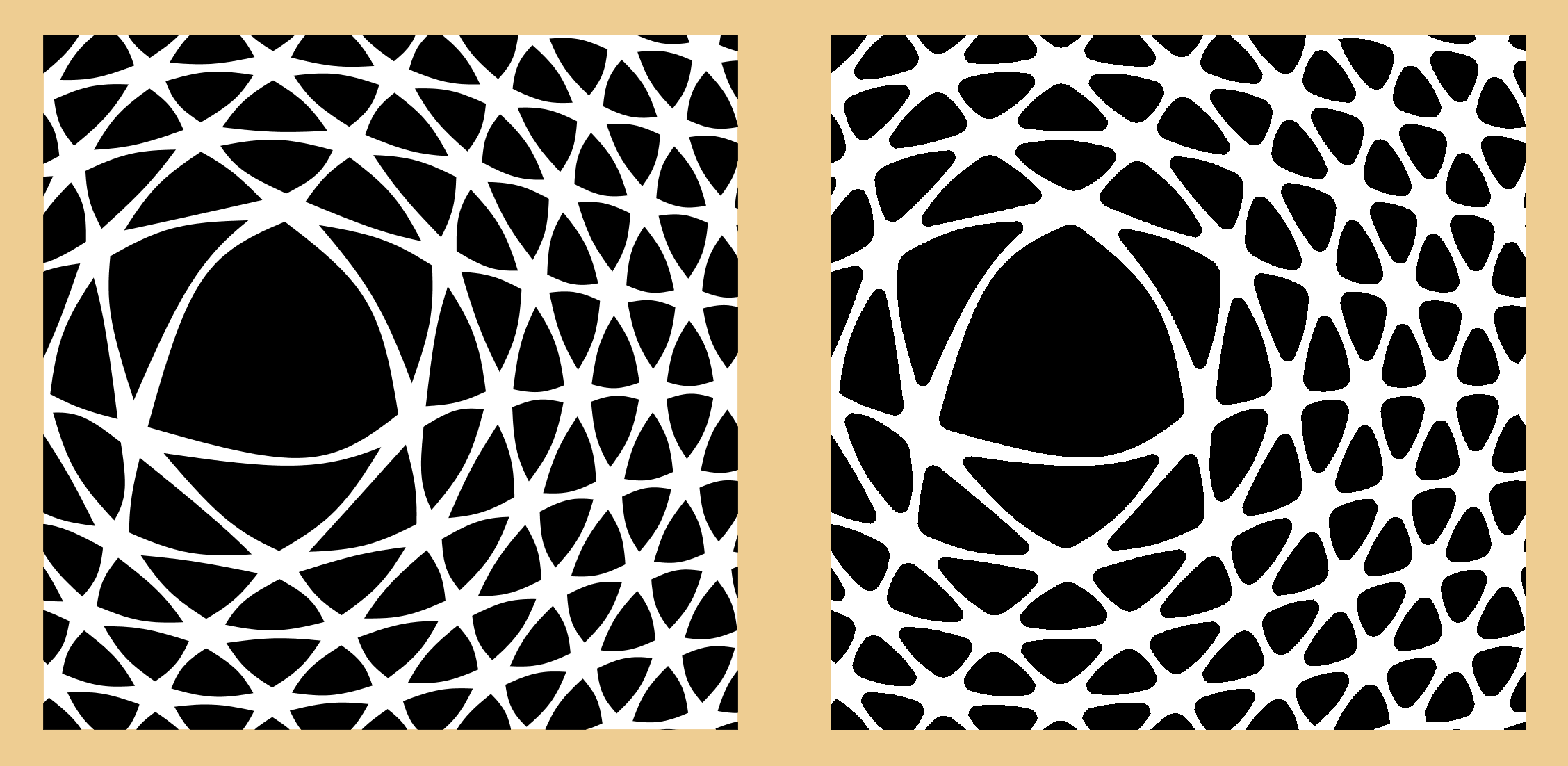
One can design variations on the glob geometry to explicitly produce smooth surfaces when two globs overlap at a common endpoint. That would handle the case of two globs, but then one would need to design new special case geometry for three globs, another special case for four, and so on. We haven't found an explicit geometric construction that will always provide smooth joins for any number of shared globs.

Happily, we can solve this problem by using implicit surfaces, like those used by blobs. In 2D, treat each pixel inside a glob as the center of a small radially symmetric blob. For each pixel outside of a glob, sum the field contributions from all in-glob pixels (in practice, we only use pixels that are within the blob's radius, since the contribution from all other pixels would be 0). Normalize the field and then threshold it, creating a smooth isosurface as shown on the right in Figure 11. In this figure, there is some thickening of the shapes due to the spread of the blob fields; one can of course draw slightly thinner shapes in the first place to compensate. The same process can be applied in 3D. This technique can be thought of as using globs as the primitives for building an implicit surface [Menon96]. Indeed, we think the match is a natural one. Globs offer us the ability to control the shape of the blend between spherical functions when we want that control, and the isosurface naturally creates other blends when we don't need to explicitly shape them.

Making Globs

My AU Library for Processing offers globs as built-in primitives. To create a glob, which the library calls an AUGlob, you specify the X and Y locations of the two circle centers centers (points C0 and C1), the radii of the two circles (r0 and r1), the X and Y locations of the two guide points (named D and Dp), and the shaping parameters $a$, $b$, $a^\prime$, and $b^\prime$, named a, b, ap, and bp.

AUGlob(PApplet theSketch, 
       PVector C0, float r0, 
       PVector C1, float r1, 
       PVector D, float a, float b, 
       PVector Dp, float ap, float bp);

Another way to specify the locations of points D and Dp uses two floats each. This con be more convenient if you're moving the glob around, and you want the points D and Dp to be the in the same relative places, but you don't want to have to recompute their locations over and over again.

In this version, to define D, you tell the system how far the point should be located on the line from C0 to C1 using the parameter dpar. The name comes from the fact that we're measuring along, or parallel to, the line from C0 to C1. The value of dpar is a number from 0 to 1, where 0 means it's just touching circle 0, and 1 means it's just touching of circle 1 (this is because placing the point D inside either circle will cause things to go haywire; if you like having things go haywire, set dpar to value less than 0 or greater than 1!). Now you can push the point away from this line by an amount dperp, also between 0 and 1. As you might guess, this name reflects the fact that we're moving the point in a direction perpendicular to the line between the circle centers. When dperp is 1, the point is pushed the same distance as the gap between the circles. To move it farther, set dperp to a larger value. To move the point in the opposite direction, set dperp to a negative value. Figure 12 illustrates the idea.

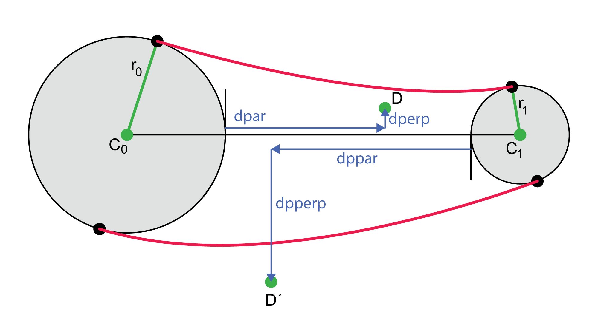
You specify the location of point Dp in the same way, with the two floats dppar and dpperp. As the arrows in the figure show, positive values of these parameters are interpreted in the directions opposite to dpar and dperp.

Note that you can bend the neck so it's all on either side of the line joining the circle centers. Just set dperp to a large positive number (say 2), and dpperp to a negative number of smaller magnitude (say -1), or vice-versa.

Here's how to make a glob using these four floats rather than explicitly locating D and Dp.

AUGlob(PApplet theSketch, 
       PVector C0, float r0, 
       PVector C1, float r1, 
       float dpar, float dperp, float a, float b, 
       float dppar, float dpperp, float ap, float bp);

As usual, use the value this for the first parameter (the one named theSketch). You can render just the neck of the glob, the two ends, or both (make sure you're inside your draw() routine!):

void render(boolean drawNeck, boolean drawCaps);

Finally, you can re-shape the glob by directly assigning to any of the parameters in the constructor. So if you wanted to change the radius of circle 0 for a glob named myGlob, you might say

myGlob.r0 = 50;

You can only change the parameters that you used when you created the glob. So if you used the first form where you explicitly provided the points D and Dp, then modifying the floats dpar, dperp, dppar, or dpperp will have no effect. Similarly, if you created the glob using the second form where you provided those floats, changing the values of D and Dp will have no effect.

If you do change any glob parameters, it's your responsibility to tell it to re-compute its shape. That way you can change lots of parameters, and then rebuild the geometry just once when you're done. Call buildGeometry() to make that happen.

myGlob.C0.x = 135;          // set the X value for the center of circle 0
myGlob.C1.x = 335;          // set the X value for the center of circle 1
myGlob.buildGeometry();     // rebuild the geometry
myGlob.render(true, true);  // and draw it

Previous Work

We note that globs have common roots with other shapes that have been discussed. The approach of [Ma12] offers an anaytic blending function of cone-spheres, with special-case geometry for creating smooth joins where two cone-spheres share a common end. Similarly, [Bastl15] offers a system for combining many cone-spheres together, but their blends are limited to cones that produce strictly convex shapes. Finally, one can consider globs to be special cases of a general swept sphere surface, as described by van Wijk [vanWijk85]. A swept sphere requires a path and a radius profile. We have found that globs offer a simpler alternative to the sometimes challenging design problem of crafting these two curves to achieve a desired shape, particularly when it comes to getting a smooth transition from the end spheres to the curved neck. We feel that a large part of the appeal of the glob primitive comes from the variety of shapes that can be produced with just a few controls, each of which has a specific geometric action.

Future Work

It's natural to think of constructing a glob with continuity in the second derivative or higher. To get C2 continuity in this geometry, we'd have to give up the freedom of placing the $F$ points where we like, which we feel would sacrifice too much of the variety and control that makes globs attractive in the first place. We are currently investigating alternative geometries that offer the same simple and direct interface controls but can provide C2 continuity. In the meantime, we note that being limited to C1 continuity isn't always such a bad thing: Max's cone-spheres are only C1 continuous and they have proven to be a popular and useful primitive. We also observe that even without a constructive guarantee of C2 continuity, most of the globs we have made are visually smooth. The examples in all the figures here are typical in this respect.

In some circumstances, rotating a glob about a line produces a useful surface of revolution. Most of the time that line will be the one that joins the two circle endpoints, but any line will do. Another way to produce a 3D model is to use an $\textit{inflation}$ technique such as [Joshi08]. We're looking at this idea and others for producing interesting 3D globs from 2D designs.

Conclusion

We've shown that with just one point and two scalars, a designer can create a graceful neck between two circles or spheres. The neck can curve inwards or outwards, and the designer can control both the location of the thinnest (or thickest) part of the neck, and how sharply the neck rises to join the circle or sphere at each end. With one more point and two more scalars, the designer can create a second Bezier curve that creates a rich variety of curved and asymmetric neck shapes. These shapes can all be promoted into 3D as collections of patches or polygons.

References

[Bastl15] Bohumir Bastl, Jiri Kosinka, and Miroslav Lavicka, "Simple and Branched Skins of Systems of Circles and Convex Shapes", Graphical Models, Volume 78, March 2015, Pages 1-9. (https://www.cl.cam.ac.uk/~jk520/papers/15BaKoLa.pdf)

[Blinn82] James F. Blinn, "A Generalization of Algebraic Surface Drawing", ACM Transactions on Graphics, Volume 1 Number 3, July 1982, Pages 235-256

[Glassner14] Andrew Glassner, "The AU Library: Equal Spacing Along Curves", Imaginary Institute Technical Note #8, December 2014 (http://imaginary-institute.com/resources/TechNote08/TechNote08.html)

[Joshi08] P. Joshi and N. Carr, "Repousse: Automatic Inflation of 2d Artwork" In Proceedings of the sixth Eurographics workshop on Sketch-Based Interfaces and Modeling, Eurographics Association, February 2008, page 49–56 (http://pushkarjoshi.org/pdf/JC_SBIM2008.pdf)

[Ma12] Yanpeng Ma, Changhe Tu, and Wenping Wang, "Distance Computation For Canal Surfaces Using Cone-Sphere Bounding Volumes", Computer Aided Geometric Design, Volume 29 Issue 5, June 2012, Pages 255-64

[Max90] Nelson Max, "Cone-Spheres", Proceedings of SIGGRAPH '90, Pages 59-62

[Menon96] Jai Menon, "An Introduction to Implicit Techniques", Course notes for Implicit Surfaces for Geometric Modeling and Computer Graphics, SIGGRAH 1996 (http://www.cs.princeton.edu/courses/archive/fall02/cs526/papers/course11sig96.pdf)

[Pomax15] Pomax, "A Primer on Bezier Curves", 2015 (http://pomax.github.io/bezierinfo/#offsetting)

[Stone89] Maureen Stone and Tony DeRose, "A Geometric Characterization of Parametric Cubic Curves", ACM Transactions on Graphics, Volume 8 Number 3, July 1989, Pages 157-163

[vanWijk85] J.J. van Wijk, "Ray Tracing Objects Defined By Sweeping A Sphere", Department of Industrial Design, Delft University of Technology, Delft, The Netherlands

[Wyvill99] Brian Wyvill and Eric Galin and Andrew Guy, "Extending The CSG Tree. Warping, Blending and Boolean Operations in an Implicit Surface Modeling System", Computer Graphics Forum, Volume 18 Number 2, June 1999, Pages 149-158

Try it out!

Go ahead and make some globs! The red dots are the centers of the circles. The orange dots are one of the curves and the teal dots are the other. The orange and teal dots with the darker centers are the narrowest (or thickest) part of the neck (these are points $D$ in Figure 2). Drag them anywhere, but things will go screwy if you put them inside one of the circles. To change the radius of the circles, click on the orange or teal dot on the perimeter of the circle (these are the points $E$ in Figure 2); you'll notice you can only drag these towards and away from the red dot. Finally, to change the way the neck forms near one of the circles, drag the colored dot at the end of a line (these are the points $F$ in Figure 2); you'll find these can only move along the line they're on.

There are a few keyboard controls:

• f: Toggle the frame (the dots and lines) on and off
• c: Toggle the caps (the circles) on and off
• n: Toggle the neck on and off
• r: Reset the shape (to start over again)

Here's the code (in Processing) for a Glob class.

class Glob {

  // The input geometry of a Glob
  PVector C0, C1;      // circle centers
  float r0, r1;        // circle radii
  PVector D, Dp;       // target points D and Dprime
  float a, b, ap, bp;  // control scalars a, b, aprime, bprime
  
  // the points we derive from the input geometry
  PVector U, V;
  PVector E0, E0p, E1, E1p, F0, F0p, F1, F1p;

  // these are for picking which tangent point we want
  final int SIDE_LEFT = -1;
  final int SIDE_RIGHT = 1;

  // make a new Glob with these parameters. Save them, then build the geometry.
  Glob(PVector _C0, float _r0, PVector _C1, float _r1, PVector _D, float _a, float _b, PVector _Dp, float _ap, float _bp) {
    C0 = _C0.get();
    C1 = _C1.get();
    r0 = _r0;
    r1 = _r1;
    D = _D.get();
    a = _a;
    b = _b;
    Dp = _Dp.get();
    ap = _ap;
    bp = _bp;
    buildGeometry();
  }
  
  // This is the heart of the class. Using the definition of Glob geometry,
  // find the coordinate system (U, V), then the tangent points E, and from them
  // the Bezier control points F.
  void buildGeometry() {
    U = PVector.sub(C1, C0);
    U.normalize();
    V = new PVector(U.y, -U.x);
    
    E0 = getTangentPoint(C0, D, r0, SIDE_RIGHT);
    E1 = getTangentPoint(C1, D, r1, SIDE_LEFT);
    E0p = getTangentPoint(C0, Dp, r0, SIDE_LEFT);
    E1p = getTangentPoint(C1, Dp, r1, SIDE_RIGHT);
  
    F0 = PVector.lerp(E0, D, a);
    F1 = PVector.lerp(E1, D, b);
    F0p = PVector.lerp(E0p, Dp, ap);
    F1p = PVector.lerp(E1p, Dp, bp);
  }
  
  // Implement Figure 3 from the tech note. Given a circle of center A and radius r,
  // a point B outside the circle, and a choice of "side", return a point on the 
  // circle that forms a tangent line to the circle with point B.
  PVector getTangentPoint(PVector A, PVector B, float r, int side) {
    PVector S = PVector.sub(B, A);
    S.normalize();
    PVector T = new PVector(S.y, -S.x);

    float ab = A.dist(B);
    float pb = sqrt(sq(ab)-sq(r));
    float beta = atan2(pb, r);
    float uscl = r * cos(beta);
    float vscl = r * sin(beta);
    PVector P0 = new PVector(A.x + (uscl*S.x) + (vscl*T.x), A.y + (uscl*S.y) + (vscl*T.y));  
    PVector P1 = new PVector(A.x + (uscl*S.x) - (vscl*T.x), A.y + (uscl*S.y) - (vscl*T.y));

    // now pick one or the other, using the sign of cross products from each P to A with S
    PVector dP0 = PVector.sub(P0, A); 
    PVector dP1 = PVector.sub(P1, A); 
    float p0sgn = S.cross(dP0).z;
    float p1sgn = S.cross(dP1).z;
    if (((p0sgn>0) && (p1sgn>0)) || ((p0sgn<0) && (p1sgn<0))) {  // this should never happen
      println("getTangentPoint: Both points are on same side of line!");
      return P0;
    }
    if (side == SIDE_RIGHT) { // the positive side is on the right
      if (p0sgn > 0) return P0;
      return P1;
    } 
    if (p0sgn < 0) return P0;
    return P1;
  }
              
  // a utility method to draw the Glob in a straightforward way
  void render(boolean drawNeck, boolean drawCaps) {
    if (drawCaps) {
      ellipse(C0.x, C0.y, 2*r0, 2*r0);
      ellipse(C1.x, C1.y, 2*r1, 2*r1);
    }
    if (drawNeck) { // this shape is what it's is all about!
      beginShape();
        vertex(E0.x, E0.y);
        bezierVertex(F0.x, F0.y, F1.x, F1.y, E1.x, E1.y);
        vertex(E1p.x, E1p.y);
        bezierVertex(F1p.x, F1p.y, F0p.x, F0p.y, E0p.x, E0p.y);
      endShape(CLOSE);
    }
  }
}